source(here::here("scripts", "R", "NbClust_indexlist.R"))
source(here::here("scripts", "R", "beta_diversity.R"))
library(phyloseq)
library(ggplot2)
Warning: package 'ggplot2' was built under R version 4.3.2library(factoextra)source(here::here("scripts", "R", "NbClust_indexlist.R"))
source(here::here("scripts", "R", "beta_diversity.R"))
library(phyloseq)
library(ggplot2)Warning: package 'ggplot2' was built under R version 4.3.2library(factoextra)getwd()[1] "/Users/marcgarel/Desktop/formation_metabarcoding_omic/scripts"output_beta <- here::here("outputs", "beta_diversity")
if (!dir.exists(output_beta)) dir.create(output_beta, recursive = TRUE)physeq <-readRDS(here::here("data","phyloseq_object_alpha_beta_div.rds"))physeq_rar <- phyloseq::rarefy_even_depth(physeq, rngseed = TRUE)Be careful when using transformation as it can distort the data. Use transformation especially for performing PCA to avoid sensitivity of double zeros (e.g Hellinger or chord transformation).
The first one you’re already see it with subsampling…
The second will employ a compositional data analysis approach and involves working with log-ratios.
A detailed discussion of compositional data analysis (CoDA) is beyond the scope of this session but just know that microbiome data is compositional since reads total is constrained by the sequencing depth. Relative abundances (proportions) are obviously constraint by a sum equal to one. This total constraint induces strong dependencies among the observed abundances of the different taxa. In fact, nor the absolute abundance (read counts) nor the relative abundance (proportion) of one taxon alone are informative of the real abundance of the taxon in the environment. Instead, they provide information on the relative measure of abundance when compared to the abundance of other taxa in the same sample. For this reason, these data fail to meet many of the assumptions of our favorite statistical methods developed for unconstrained random variables. Working with ratios of compositional elements lets us transform these data to the Euclidian space and apply our favorite methods. There are different types of log-ratio “transformations” including the additive log-ratio, centered log-ratio, and isometric log-ratio transforms. Find more information here, here and here
Let’s perform the CLR transformation
 # we first replace the zeros using
 # the Count Zero Multiplicative approach (other alternative pseudocount)
tmp <- zCompositions::cmultRepl(physeq@otu_table,
                                method = "CZM",
                                label = 0, z.warning=1)
head(tmp)
ASV1 ASV2 ASV3 ASV4 ASV5 ASV6
S11B 0.11292000 0.0241282051 0.0820358974 0.0675589744 0.08396615 0.0386051282
S1B 0.07451522 0.0003882915 0.0255798501 0.0003882915 0.05672054 0.0533840350
S2B 0.04517311 0.0003639418 0.0367688090 0.0157580610 0.04412257 0.0546279449
S2S 0.09868414 0.0833545658 0.0728154827 0.0114971815 0.09485175 0.0411982337
S3B 0.06291984 0.0003701595 0.0341260164 0.0003701595 0.05225546 0.0778499748
S3S 0.08531780 0.0105330619 0.0003655793 0.0210661238 0.03791902 0.0003655793
ASV7 ASV8 ASV9 ASV10 ASV11
S11B 0.0550123077 0.0328143590 0.0395702564 0.0003333333 0.0003333333
S1B 0.0003882915 0.0003882915 0.0300285197 0.0645057089 0.0622813741
S2B 0.0003639418 0.0003639418 0.0003639418 0.0451731082 0.0630322441
S2S 0.0344915445 0.0689830889 0.0440725290 0.0003306205 0.0003306205
S3B 0.0003701595 0.0003701595 0.0003701595 0.0607869667 0.0725177848
S3S 0.0003655793 0.0003655793 0.0003655793 0.0526653094 0.0547719218
ASV12 ASV13 ASV14 ASV15 ASV16
S11B 0.0003333333 0.0193025641 0.0003333333 0.0241282051 0.0003333333
S1B 0.0578327046 0.0003882915 0.0003882915 0.0003882915 0.0522718676
S2B 0.0304655846 0.0031516122 0.0003639418 0.0003639418 0.0577795571
S2S 0.0003306205 0.0574859074 0.0003306205 0.0364077414 0.0003306205
S3B 0.0618534047 0.0003701595 0.0003701595 0.0003701595 0.0501225865
S3S 0.1042773126 0.0003655793 0.0003655793 0.0003655793 0.0600384527
ASV17 ASV18 ASV19 ASV20 ASV21
S11B 0.0003333333 0.0003333333 0.0347446154 0.0569425641 0.0212328205
S1B 0.0003882915 0.0400380262 0.0003882915 0.0003882915 0.0003882915
S2B 0.0003639418 0.0451731082 0.0003639418 0.0003639418 0.0252128976
S2S 0.0003306205 0.0003306205 0.0239524614 0.0354496429 0.0258686583
S3B 0.0003701595 0.0469232725 0.0003701595 0.0003701595 0.0362588924
S3S 0.0663582899 0.0326524918 0.0003655793 0.0003655793 0.0003655793
ASV22 ASV23 ASV24 ASV25 ASV26
S11B 0.0003333333 0.0003333333 0.0241282051 0.0003333333 0.0057907692
S1B 0.0003882915 0.0003882915 0.0003882915 0.0003882915 0.0003882915
S2B 0.0294150472 0.0325666594 0.0168085984 0.0003639418 0.0003639418
S2S 0.0003306205 0.0003306205 0.0210781661 0.0003306205 0.0019161969
S3B 0.0287938263 0.0277273883 0.0003701595 0.0003701595 0.0003701595
S3S 0.0379190228 0.0284392671 0.0003655793 0.0003655793 0.0063198371
ASV27 ASV28 ASV29 ASV30 ASV31
S11B 0.0328143590 0.0003333333 0.0003333333 0.0003333333 0.0003333333
S1B 0.0003882915 0.0003882915 0.0003882915 0.0003882915 0.0003882915
S2B 0.0003639418 0.0745881555 0.0003639418 0.0105053740 0.0003639418
S2S 0.0067066892 0.0003306205 0.0172457722 0.0003306205 0.0003306205
S3B 0.0003701595 0.0003701595 0.0003701595 0.0351924544 0.0003701595
S3S 0.0003655793 0.0231727361 0.0003655793 0.0179062052 0.0003655793
ASV32 ASV33 ASV34 ASV35 ASV36
S11B 0.0003333333 0.0241282051 0.0003333333 0.0003333333 0.0164071795
S1B 0.0344771893 0.0003882915 0.0722908807 0.0367015240 0.0003882915
S2B 0.0115559114 0.0052526870 0.0003639418 0.0157580610 0.0003639418
S2S 0.0003306205 0.0134133784 0.0003306205 0.0003306205 0.0003306205
S3B 0.0106643801 0.0003701595 0.0586540906 0.0223951982 0.0003701595
S3S 0.0389723290 0.0157995928 0.0003655793 0.0073731433 0.0003655793
ASV37 ASV38 ASV39 ASV40 ASV41
S11B 0.0115815385 0.0003333333 0.0003333333 0.0003333333 0.0086861538
S1B 0.0055608370 0.0003882915 0.0003882915 0.0003882915 0.0003882915
S2B 0.0003639418 0.0003639418 0.0003639418 0.0003639418 0.0199602106
S2S 0.0038323938 0.0003306205 0.0003306205 0.0003306205 0.0162876738
S3B 0.0053321901 0.0003701595 0.0003701595 0.0003701595 0.0003701595
S3S 0.0558252280 0.0003655793 0.0003655793 0.0003655793 0.0003655793
ASV42 ASV43 ASV44 ASV45 ASV46
S11B 0.0003333333 0.0003333333 0.0003333333 0.0183374359 0.0003333333
S1B 0.0003882915 0.0003882915 0.0003882915 0.0003882915 0.0522718676
S2B 0.0003639418 0.0003639418 0.0003639418 0.0003639418 0.0003639418
S2S 0.0003306205 0.0057485907 0.0003306205 0.0114971815 0.0003306205
S3B 0.0003701595 0.0003701595 0.0003701595 0.0003701595 0.0003701595
S3S 0.0003655793 0.0003655793 0.0003655793 0.0003655793 0.0003655793
ASV47 ASV48 ASV49 ASV50 ASV51
S11B 0.0003333333 0.0003333333 0.0003333333 0.0260584615 0.0048256410
S1B 0.0003882915 0.0003882915 0.0003882915 0.0003882915 0.0055608370
S2B 0.0003639418 0.0003639418 0.0210107480 0.0003639418 0.0003639418
S2S 0.0003306205 0.0003306205 0.0003306205 0.0277848553 0.0057485907
S3B 0.0003701595 0.0003701595 0.0149301322 0.0003701595 0.0003701595
S3S 0.0003655793 0.0003655793 0.0147462866 0.0003655793 0.0031599186
ASV52 ASV53 ASV54 ASV55 ASV56
S11B 0.0003333333 0.0003333333 0.0028953846 0.0003333333 0.0003333333
S1B 0.0003882915 0.0133460087 0.0003882915 0.0111216740 0.0003882915
S2B 0.0003639418 0.0178591358 0.0003639418 0.0315161220 0.0003639418
S2S 0.0003306205 0.0003306205 0.0067066892 0.0003306205 0.0076647877
S3B 0.0003701595 0.0138636941 0.0003701595 0.0095979421 0.0003701595
S3S 0.0003655793 0.0115863681 0.0003655793 0.0003655793 0.0003655793
ASV57 ASV58 ASV59 ASV60 ASV61
S11B 0.0003333333 0.0003333333 0.0086861538 0.0003333333 0.0003333333
S1B 0.0003882915 0.0122338413 0.0003882915 0.0003882915 0.0003882915
S2B 0.0003639418 0.0157580610 0.0003639418 0.0126064488 0.0003639418
S2S 0.0003306205 0.0003306205 0.0067066892 0.0003306205 0.0003306205
S3B 0.0003701595 0.0003701595 0.0003701595 0.0003701595 0.0003701595
S3S 0.0003655793 0.0003655793 0.0003655793 0.0084264495 0.0003655793
ASV62 ASV63 ASV64 ASV65 ASV66
S11B 0.0003333333 0.0125466667 0.0003333333 0.0003333333 0.0003333333
S1B 0.0003882915 0.0003882915 0.0003882915 0.0003882915 0.0003882915
S2B 0.0003639418 0.0003639418 0.0147075236 0.0003639418 0.0003639418
S2S 0.0003306205 0.0153295753 0.0019161969 0.0003306205 0.0003306205
S3B 0.0003701595 0.0003701595 0.0159965702 0.0003701595 0.0003701595
S3S 0.0003655793 0.0003655793 0.0003655793 0.0052665309 0.0003655793
ASV67 ASV68 ASV69 ASV70 ASV71
S11B 0.0003333333 0.0003333333 0.0003333333 0.0003333333 0.0003333333
S1B 0.0003882915 0.0003882915 0.0003882915 0.0003882915 0.0003882915
S2B 0.0003639418 0.0003639418 0.0003639418 0.0003639418 0.0003639418
S2S 0.0095809846 0.0003306205 0.0003306205 0.0095809846 0.0003306205
S3B 0.0003701595 0.0003701595 0.0003701595 0.0003701595 0.0003701595
S3S 0.0003655793 0.0003655793 0.0003655793 0.0003655793 0.0003655793
ASV72 ASV73 ASV74 ASV75 ASV76
S11B 0.0003333333 0.0003333333 0.0003333333 0.0003333333 0.0003333333
S1B 0.0003882915 0.0003882915 0.0003882915 0.0003882915 0.0322528545
S2B 0.0136569862 0.0115559114 0.0073537618 0.0003639418 0.0003639418
S2S 0.0003306205 0.0003306205 0.0003306205 0.0003306205 0.0003306205
S3B 0.0117308181 0.0003701595 0.0063986281 0.0003701595 0.0003701595
S3S 0.0003655793 0.0200128176 0.0052665309 0.0003655793 0.0003655793
ASV77 ASV78 ASV79 ASV80 ASV81
S11B 0.0003333333 0.0115815385 0.0003333333 0.0003333333 0.0003333333
S1B 0.0003882915 0.0003882915 0.0003882915 0.0003882915 0.0003882915
S2B 0.0003639418 0.0003639418 0.0003639418 0.0003639418 0.0003639418
S2S 0.0003306205 0.0003306205 0.0003306205 0.0003306205 0.0003306205
S3B 0.0003701595 0.0003701595 0.0003701595 0.0003701595 0.0003701595
S3S 0.0003655793 0.0003655793 0.0003655793 0.0003655793 0.0003655793
ASV82 ASV83 ASV84 ASV85 ASV86
S11B 0.0003333333 0.0003333333 0.0003333333 0.0003333333 0.0003333333
S1B 0.0122338413 0.0003882915 0.0003882915 0.0003882915 0.0003882915
S2B 0.0003639418 0.0003639418 0.0003639418 0.0003639418 0.0105053740
S2S 0.0003306205 0.0003306205 0.0003306205 0.0003306205 0.0003306205
S3B 0.0159965702 0.0003701595 0.0003701595 0.0003701595 0.0063986281
S3S 0.0003655793 0.0003655793 0.0003655793 0.0003655793 0.0073731433
ASV87 ASV88 ASV89 ASV90 ASV91
S11B 0.0003333333 0.0048256410 0.0003333333 0.0003333333 0.0003333333
S1B 0.0003882915 0.0003882915 0.0003882915 0.0003882915 0.0003882915
S2B 0.0003639418 0.0003639418 0.0003639418 0.0003639418 0.0084042992
S2S 0.0003306205 0.0003306205 0.0003306205 0.0003306205 0.0057485907
S3B 0.0003701595 0.0003701595 0.0095979421 0.0003701595 0.0003701595
S3S 0.0003655793 0.0003655793 0.0136929804 0.0003655793 0.0003655793
ASV92 ASV93 ASV94 ASV95 ASV96
S11B 0.0003333333 0.0003333333 0.0003333333 0.0003333333 0.0003333333
S1B 0.0211311805 0.0003882915 0.0003882915 0.0003882915 0.0003882915
S2B 0.0003639418 0.0073537618 0.0003639418 0.0003639418 0.0003639418
S2S 0.0003306205 0.0003306205 0.0003306205 0.0003306205 0.0003306205
S3B 0.0003701595 0.0003701595 0.0003701595 0.0003701595 0.0003701595
S3S 0.0003655793 0.0073731433 0.0003655793 0.0003655793 0.0003655793
ASV97 ASV98 ASV99 ASV100 ASV101
S11B 0.0003333333 0.0003333333 0.0003333333 0.0003333333 0.0003333333
S1B 0.0003882915 0.0066730044 0.0003882915 0.0003882915 0.0003882915
S2B 0.0003639418 0.0003639418 0.0168085984 0.0084042992 0.0003639418
S2S 0.0003306205 0.0003306205 0.0003306205 0.0003306205 0.0003306205
S3B 0.0003701595 0.0003701595 0.0003701595 0.0003701595 0.0003701595
S3S 0.0003655793 0.0003655793 0.0003655793 0.0003655793 0.0168528990
ASV102 ASV103 ASV104 ASV105 ASV106
S11B 0.0003333333 0.0003333333 0.0003333333 0.0048256410 0.0038605128
S1B 0.0003882915 0.0003882915 0.0003882915 0.0003882915 0.0003882915
S2B 0.0003639418 0.0003639418 0.0003639418 0.0003639418 0.0003639418
S2S 0.0003306205 0.0003306205 0.0003306205 0.0003306205 0.0003306205
S3B 0.0003701595 0.0003701595 0.0003701595 0.0003701595 0.0003701595
S3S 0.0003655793 0.0003655793 0.0003655793 0.0003655793 0.0003655793
ASV107 ASV108 ASV109 ASV110 ASV111
S11B 0.0003333333 0.0003333333 0.0003333333 0.0003333333 0.0003333333
S1B 0.0166825109 0.0003882915 0.0003882915 0.0003882915 0.0003882915
S2B 0.0003639418 0.0157580610 0.0003639418 0.0003639418 0.0003639418
S2S 0.0003306205 0.0003306205 0.0003306205 0.0003306205 0.0003306205
S3B 0.0003701595 0.0003701595 0.0003701595 0.0003701595 0.0003701595
S3S 0.0003655793 0.0003655793 0.0147462866 0.0147462866 0.0003655793
ASV112 ASV113 ASV114 ASV115 ASV116
S11B 0.0003333333 0.0003333333 0.0003333333 0.0003333333 0.0003333333
S1B 0.0077851718 0.0003882915 0.0003882915 0.0003882915 0.0003882915
S2B 0.0003639418 0.0003639418 0.0003639418 0.0003639418 0.0003639418
S2S 0.0003306205 0.0003306205 0.0003306205 0.0003306205 0.0003306205
S3B 0.0063986281 0.0138636941 0.0003701595 0.0003701595 0.0003701595
S3S 0.0003655793 0.0003655793 0.0003655793 0.0003655793 0.0003655793
ASV117 ASV118 ASV119 ASV120 ASV121
S11B 0.0003333333 0.0003333333 0.0003333333 0.0003333333 0.0003333333
S1B 0.0003882915 0.0003882915 0.0003882915 0.0066730044 0.0003882915
S2B 0.0126064488 0.0094548366 0.0003639418 0.0003639418 0.0042021496
S2S 0.0003306205 0.0003306205 0.0003306205 0.0003306205 0.0003306205
S3B 0.0003701595 0.0003701595 0.0003701595 0.0003701595 0.0074650661
S3S 0.0003655793 0.0003655793 0.0003655793 0.0052665309 0.0003655793
ASV122 ASV123 ASV124 ASV125 ASV126
S11B 0.0003333333 0.0003333333 0.0003333333 0.0096512821 0.0077210256
S1B 0.0003882915 0.0003882915 0.0003882915 0.0003882915 0.0003882915
S2B 0.0003639418 0.0003639418 0.0003639418 0.0003639418 0.0021010748
S2S 0.0003306205 0.0003306205 0.0003306205 0.0003306205 0.0003306205
S3B 0.0003701595 0.0003701595 0.0003701595 0.0003701595 0.0003701595
S3S 0.0003655793 0.0003655793 0.0003655793 0.0003655793 0.0003655793
ASV127 ASV128 ASV129 ASV130 ASV131
S11B 0.0003333333 0.0003333333 0.0003333333 0.0003333333 0.0003333333
S1B 0.0003882915 0.0003882915 0.0003882915 0.0003882915 0.0003882915
S2B 0.0003639418 0.0003639418 0.0003639418 0.0003639418 0.0003639418
S2S 0.0003306205 0.0003306205 0.0003306205 0.0003306205 0.0003306205
S3B 0.0106643801 0.0053321901 0.0042657520 0.0003701595 0.0003701595
S3S 0.0003655793 0.0003655793 0.0063198371 0.0003655793 0.0003655793
ASV132 ASV133 ASV134 ASV135 ASV136
S11B 0.0003333333 0.0003333333 0.0003333333 0.0003333333 0.0003333333
S1B 0.0003882915 0.0003882915 0.0100095066 0.0100095066 0.0003882915
S2B 0.0003639418 0.0003639418 0.0003639418 0.0003639418 0.0003639418
S2S 0.0003306205 0.0003306205 0.0003306205 0.0003306205 0.0019161969
S3B 0.0003701595 0.0003701595 0.0003701595 0.0003701595 0.0003701595
S3S 0.0003655793 0.0003655793 0.0003655793 0.0003655793 0.0003655793
ASV137 ASV138 ASV139 ASV140 ASV141
S11B 0.0003333333 0.0003333333 0.0003333333 0.0003333333 0.0003333333
S1B 0.0003882915 0.0003882915 0.0003882915 0.0003882915 0.0003882915
S2B 0.0003639418 0.0003639418 0.0003639418 0.0003639418 0.0003639418
S2S 0.0003306205 0.0003306205 0.0003306205 0.0003306205 0.0003306205
S3B 0.0003701595 0.0003701595 0.0003701595 0.0003701595 0.0003701595
S3S 0.0003655793 0.0003655793 0.0003655793 0.0003655793 0.0003655793
ASV142 ASV143 ASV144 ASV145 ASV146
S11B 0.0003333333 0.0003333333 0.0003333333 0.0003333333 0.0003333333
S1B 0.0003882915 0.0003882915 0.0088973392 0.0088973392 0.0003882915
S2B 0.0003639418 0.0003639418 0.0003639418 0.0003639418 0.0003639418
S2S 0.0003306205 0.0003306205 0.0003306205 0.0003306205 0.0076647877
S3B 0.0003701595 0.0003701595 0.0003701595 0.0003701595 0.0003701595
S3S 0.0003655793 0.0003655793 0.0003655793 0.0003655793 0.0003655793
ASV147 ASV148 ASV149 ASV150 ASV151
S11B 0.0003333333 0.0003333333 0.0003333333 0.0003333333 0.0003333333
S1B 0.0003882915 0.0003882915 0.0003882915 0.0003882915 0.0003882915
S2B 0.0003639418 0.0003639418 0.0003639418 0.0003639418 0.0003639418
S2S 0.0003306205 0.0003306205 0.0003306205 0.0003306205 0.0003306205
S3B 0.0003701595 0.0003701595 0.0003701595 0.0003701595 0.0003701595
S3S 0.0084264495 0.0003655793 0.0003655793 0.0003655793 0.0003655793
ASV152 ASV153 ASV154 ASV155 ASV156
S11B 0.0003333333 0.0003333333 0.0003333333 0.0003333333 0.0003333333
S1B 0.0003882915 0.0003882915 0.0077851718 0.0003882915 0.0003882915
S2B 0.0003639418 0.0003639418 0.0003639418 0.0073537618 0.0003639418
S2S 0.0003306205 0.0003306205 0.0003306205 0.0003306205 0.0003306205
S3B 0.0003701595 0.0003701595 0.0003701595 0.0003701595 0.0074650661
S3S 0.0003655793 0.0003655793 0.0003655793 0.0003655793 0.0003655793
ASV157 ASV158 ASV159 ASV160 ASV161
S11B 0.0003333333 0.0003333333 0.0003333333 0.0003333333 0.0003333333
S1B 0.0003882915 0.0003882915 0.0003882915 0.0003882915 0.0003882915
S2B 0.0003639418 0.0003639418 0.0003639418 0.0003639418 0.0003639418
S2S 0.0003306205 0.0003306205 0.0003306205 0.0003306205 0.0003306205
S3B 0.0003701595 0.0003701595 0.0003701595 0.0003701595 0.0003701595
S3S 0.0003655793 0.0003655793 0.0003655793 0.0003655793 0.0003655793
ASV162 ASV163 ASV164 ASV165 ASV166
S11B 0.0003333333 0.0003333333 0.0003333333 0.0003333333 0.0003333333
S1B 0.0003882915 0.0003882915 0.0003882915 0.0066730044 0.0066730044
S2B 0.0003639418 0.0003639418 0.0003639418 0.0003639418 0.0003639418
S2S 0.0003306205 0.0003306205 0.0003306205 0.0003306205 0.0003306205
S3B 0.0003701595 0.0003701595 0.0003701595 0.0003701595 0.0003701595
S3S 0.0003655793 0.0003655793 0.0003655793 0.0003655793 0.0003655793
ASV167 ASV168 ASV169 ASV170 ASV171
S11B 0.0003333333 0.0003333333 0.0003333333 0.0003333333 0.0003333333
S1B 0.0003882915 0.0003882915 0.0003882915 0.0003882915 0.0003882915
S2B 0.0003639418 0.0003639418 0.0003639418 0.0003639418 0.0003639418
S2S 0.0003306205 0.0003306205 0.0003306205 0.0003306205 0.0003306205
S3B 0.0063986281 0.0021328760 0.0003701595 0.0003701595 0.0003701595
S3S 0.0003655793 0.0003655793 0.0063198371 0.0003655793 0.0003655793
ASV172 ASV173 ASV174 ASV175 ASV176
S11B 0.0003333333 0.0003333333 0.0003333333 0.0003333333 0.0003333333
S1B 0.0003882915 0.0055608370 0.0003882915 0.0003882915 0.0003882915
S2B 0.0003639418 0.0003639418 0.0003639418 0.0003639418 0.0003639418
S2S 0.0003306205 0.0003306205 0.0047904923 0.0003306205 0.0003306205
S3B 0.0003701595 0.0003701595 0.0003701595 0.0053321901 0.0053321901
S3S 0.0003655793 0.0003655793 0.0003655793 0.0003655793 0.0003655793
ASV177 ASV178 ASV179 ASV180 ASV181
S11B 0.0003333333 0.0003333333 0.0003333333 0.0003333333 0.0003333333
S1B 0.0003882915 0.0003882915 0.0003882915 0.0003882915 0.0003882915
S2B 0.0003639418 0.0003639418 0.0003639418 0.0003639418 0.0003639418
S2S 0.0003306205 0.0003306205 0.0003306205 0.0003306205 0.0003306205
S3B 0.0003701595 0.0003701595 0.0003701595 0.0003701595 0.0003701595
S3S 0.0003655793 0.0003655793 0.0003655793 0.0003655793 0.0003655793
ASV182 ASV183 ASV184 ASV185 ASV186
S11B 0.0003333333 0.0038605128 0.0003333333 0.0003333333 0.0003333333
S1B 0.0003882915 0.0003882915 0.0003882915 0.0003882915 0.0003882915
S2B 0.0003639418 0.0003639418 0.0042021496 0.0003639418 0.0003639418
S2S 0.0003306205 0.0003306205 0.0003306205 0.0038323938 0.0003306205
S3B 0.0003701595 0.0003701595 0.0003701595 0.0003701595 0.0042657520
S3S 0.0003655793 0.0003655793 0.0003655793 0.0003655793 0.0003655793
ASV187 ASV188 ASV189 ASV190 ASV191
S11B 0.0003333333 0.0003333333 0.0003333333 0.0003333333 0.0003333333
S1B 0.0003882915 0.0003882915 0.0003882915 0.0003882915 0.0003882915
S2B 0.0003639418 0.0003639418 0.0003639418 0.0003639418 0.0003639418
S2S 0.0003306205 0.0003306205 0.0003306205 0.0003306205 0.0003306205
S3B 0.0003701595 0.0003701595 0.0003701595 0.0003701595 0.0003701595
S3S 0.0042132248 0.0003655793 0.0003655793 0.0003655793 0.0003655793
ASV192 ASV193 ASV194 ASV195 ASV196
S11B 0.0003333333 0.0003333333 0.0003333333 0.0028953846 0.0003333333
S1B 0.0003882915 0.0003882915 0.0003882915 0.0003882915 0.0003882915
S2B 0.0003639418 0.0003639418 0.0003639418 0.0003639418 0.0003639418
S2S 0.0003306205 0.0003306205 0.0003306205 0.0003306205 0.0003306205
S3B 0.0003701595 0.0003701595 0.0003701595 0.0003701595 0.0031993140
S3S 0.0003655793 0.0003655793 0.0003655793 0.0003655793 0.0003655793
ASV197 ASV198 ASV199 ASV200 ASV201
S11B 0.0003333333 0.0003333333 0.0003333333 0.0003333333 0.0003333333
S1B 0.0003882915 0.0003882915 0.0003882915 0.0003882915 0.0003882915
S2B 0.0003639418 0.0003639418 0.0003639418 0.0003639418 0.0003639418
S2S 0.0003306205 0.0003306205 0.0003306205 0.0003306205 0.0003306205
S3B 0.0031993140 0.0003701595 0.0003701595 0.0003701595 0.0003701595
S3S 0.0003655793 0.0031599186 0.0003655793 0.0003655793 0.0003655793
ASV202 ASV203 ASV204 ASV205 ASV206
S11B 0.0019302564 0.0003333333 0.0003333333 0.0003333333 0.0003333333
S1B 0.0003882915 0.0022243348 0.0003882915 0.0003882915 0.0003882915
S2B 0.0003639418 0.0003639418 0.0021010748 0.0003639418 0.0003639418
S2S 0.0003306205 0.0003306205 0.0003306205 0.0003306205 0.0003306205
S3B 0.0003701595 0.0003701595 0.0003701595 0.0021328760 0.0003701595
S3S 0.0003655793 0.0003655793 0.0003655793 0.0003655793 0.0021066124
ASV207 ASV208 ASV209 ASV210 ASV211
S11B 0.0003333333 0.0003333333 0.0003333333 0.0003333333 0.0003333333
S1B 0.0003882915 0.0003882915 0.0003882915 0.0003882915 0.0003882915
S2B 0.0003639418 0.0003639418 0.0003639418 0.0003639418 0.0003639418
S2S 0.0003306205 0.0003306205 0.0003306205 0.0003306205 0.0003306205
S3B 0.0003701595 0.0003701595 0.0003701595 0.0003701595 0.0003701595
S3S 0.0003655793 0.0003655793 0.0003655793 0.0003655793 0.0003655793
ASV212 ASV213
S11B 0.0003333333 0.0003333333
S1B 0.0003882915 0.0003882915
S2B 0.0003639418 0.0003639418
S2S 0.0003306205 0.0003306205
S3B 0.0003701595 0.0003701595
S3S 0.0003655793 0.0003655793colSums(t(tmp))S11B S1B S2B S2S S3B S3S S4B S4S S5B S5S S6B S6S S7B S7S S8B S8S
1 1 1 1 1 1 1 1 1 1 1 1 1 1 1 1
S9B S9S
1 1 #create a new phyloseq object with future CLR tranformed counts
physeq_clr <- physeq
#replace the otu_table by the tmp one
otu_table(physeq_clr) <- otu_table(tmp,taxa_are_rows = FALSE)
head(physeq_clr@otu_table)OTU Table: [213 taxa and 6 samples]
taxa are columns
           ASV1         ASV2         ASV3         ASV4       ASV5         ASV6
S11B 0.11292000 0.0241282051 0.0820358974 0.0675589744 0.08396615 0.0386051282
S1B  0.07451522 0.0003882915 0.0255798501 0.0003882915 0.05672054 0.0533840350
S2B  0.04517311 0.0003639418 0.0367688090 0.0157580610 0.04412257 0.0546279449
S2S  0.09868414 0.0833545658 0.0728154827 0.0114971815 0.09485175 0.0411982337
S3B  0.06291984 0.0003701595 0.0341260164 0.0003701595 0.05225546 0.0778499748
S3S  0.08531780 0.0105330619 0.0003655793 0.0210661238 0.03791902 0.0003655793
             ASV7         ASV8         ASV9        ASV10        ASV11
S11B 0.0550123077 0.0328143590 0.0395702564 0.0003333333 0.0003333333
S1B  0.0003882915 0.0003882915 0.0300285197 0.0645057089 0.0622813741
S2B  0.0003639418 0.0003639418 0.0003639418 0.0451731082 0.0630322441
S2S  0.0344915445 0.0689830889 0.0440725290 0.0003306205 0.0003306205
S3B  0.0003701595 0.0003701595 0.0003701595 0.0607869667 0.0725177848
S3S  0.0003655793 0.0003655793 0.0003655793 0.0526653094 0.0547719218
            ASV12        ASV13        ASV14        ASV15        ASV16
S11B 0.0003333333 0.0193025641 0.0003333333 0.0241282051 0.0003333333
S1B  0.0578327046 0.0003882915 0.0003882915 0.0003882915 0.0522718676
S2B  0.0304655846 0.0031516122 0.0003639418 0.0003639418 0.0577795571
S2S  0.0003306205 0.0574859074 0.0003306205 0.0364077414 0.0003306205
S3B  0.0618534047 0.0003701595 0.0003701595 0.0003701595 0.0501225865
S3S  0.1042773126 0.0003655793 0.0003655793 0.0003655793 0.0600384527
            ASV17        ASV18        ASV19        ASV20        ASV21
S11B 0.0003333333 0.0003333333 0.0347446154 0.0569425641 0.0212328205
S1B  0.0003882915 0.0400380262 0.0003882915 0.0003882915 0.0003882915
S2B  0.0003639418 0.0451731082 0.0003639418 0.0003639418 0.0252128976
S2S  0.0003306205 0.0003306205 0.0239524614 0.0354496429 0.0258686583
S3B  0.0003701595 0.0469232725 0.0003701595 0.0003701595 0.0362588924
S3S  0.0663582899 0.0326524918 0.0003655793 0.0003655793 0.0003655793
            ASV22        ASV23        ASV24        ASV25        ASV26
S11B 0.0003333333 0.0003333333 0.0241282051 0.0003333333 0.0057907692
S1B  0.0003882915 0.0003882915 0.0003882915 0.0003882915 0.0003882915
S2B  0.0294150472 0.0325666594 0.0168085984 0.0003639418 0.0003639418
S2S  0.0003306205 0.0003306205 0.0210781661 0.0003306205 0.0019161969
S3B  0.0287938263 0.0277273883 0.0003701595 0.0003701595 0.0003701595
S3S  0.0379190228 0.0284392671 0.0003655793 0.0003655793 0.0063198371
            ASV27        ASV28        ASV29        ASV30        ASV31
S11B 0.0328143590 0.0003333333 0.0003333333 0.0003333333 0.0003333333
S1B  0.0003882915 0.0003882915 0.0003882915 0.0003882915 0.0003882915
S2B  0.0003639418 0.0745881555 0.0003639418 0.0105053740 0.0003639418
S2S  0.0067066892 0.0003306205 0.0172457722 0.0003306205 0.0003306205
S3B  0.0003701595 0.0003701595 0.0003701595 0.0351924544 0.0003701595
S3S  0.0003655793 0.0231727361 0.0003655793 0.0179062052 0.0003655793
            ASV32        ASV33        ASV34        ASV35        ASV36
S11B 0.0003333333 0.0241282051 0.0003333333 0.0003333333 0.0164071795
S1B  0.0344771893 0.0003882915 0.0722908807 0.0367015240 0.0003882915
S2B  0.0115559114 0.0052526870 0.0003639418 0.0157580610 0.0003639418
S2S  0.0003306205 0.0134133784 0.0003306205 0.0003306205 0.0003306205
S3B  0.0106643801 0.0003701595 0.0586540906 0.0223951982 0.0003701595
S3S  0.0389723290 0.0157995928 0.0003655793 0.0073731433 0.0003655793
            ASV37        ASV38        ASV39        ASV40        ASV41
S11B 0.0115815385 0.0003333333 0.0003333333 0.0003333333 0.0086861538
S1B  0.0055608370 0.0003882915 0.0003882915 0.0003882915 0.0003882915
S2B  0.0003639418 0.0003639418 0.0003639418 0.0003639418 0.0199602106
S2S  0.0038323938 0.0003306205 0.0003306205 0.0003306205 0.0162876738
S3B  0.0053321901 0.0003701595 0.0003701595 0.0003701595 0.0003701595
S3S  0.0558252280 0.0003655793 0.0003655793 0.0003655793 0.0003655793
            ASV42        ASV43        ASV44        ASV45        ASV46
S11B 0.0003333333 0.0003333333 0.0003333333 0.0183374359 0.0003333333
S1B  0.0003882915 0.0003882915 0.0003882915 0.0003882915 0.0522718676
S2B  0.0003639418 0.0003639418 0.0003639418 0.0003639418 0.0003639418
S2S  0.0003306205 0.0057485907 0.0003306205 0.0114971815 0.0003306205
S3B  0.0003701595 0.0003701595 0.0003701595 0.0003701595 0.0003701595
S3S  0.0003655793 0.0003655793 0.0003655793 0.0003655793 0.0003655793
            ASV47        ASV48        ASV49        ASV50        ASV51
S11B 0.0003333333 0.0003333333 0.0003333333 0.0260584615 0.0048256410
S1B  0.0003882915 0.0003882915 0.0003882915 0.0003882915 0.0055608370
S2B  0.0003639418 0.0003639418 0.0210107480 0.0003639418 0.0003639418
S2S  0.0003306205 0.0003306205 0.0003306205 0.0277848553 0.0057485907
S3B  0.0003701595 0.0003701595 0.0149301322 0.0003701595 0.0003701595
S3S  0.0003655793 0.0003655793 0.0147462866 0.0003655793 0.0031599186
            ASV52        ASV53        ASV54        ASV55        ASV56
S11B 0.0003333333 0.0003333333 0.0028953846 0.0003333333 0.0003333333
S1B  0.0003882915 0.0133460087 0.0003882915 0.0111216740 0.0003882915
S2B  0.0003639418 0.0178591358 0.0003639418 0.0315161220 0.0003639418
S2S  0.0003306205 0.0003306205 0.0067066892 0.0003306205 0.0076647877
S3B  0.0003701595 0.0138636941 0.0003701595 0.0095979421 0.0003701595
S3S  0.0003655793 0.0115863681 0.0003655793 0.0003655793 0.0003655793
            ASV57        ASV58        ASV59        ASV60        ASV61
S11B 0.0003333333 0.0003333333 0.0086861538 0.0003333333 0.0003333333
S1B  0.0003882915 0.0122338413 0.0003882915 0.0003882915 0.0003882915
S2B  0.0003639418 0.0157580610 0.0003639418 0.0126064488 0.0003639418
S2S  0.0003306205 0.0003306205 0.0067066892 0.0003306205 0.0003306205
S3B  0.0003701595 0.0003701595 0.0003701595 0.0003701595 0.0003701595
S3S  0.0003655793 0.0003655793 0.0003655793 0.0084264495 0.0003655793
            ASV62        ASV63        ASV64        ASV65        ASV66
S11B 0.0003333333 0.0125466667 0.0003333333 0.0003333333 0.0003333333
S1B  0.0003882915 0.0003882915 0.0003882915 0.0003882915 0.0003882915
S2B  0.0003639418 0.0003639418 0.0147075236 0.0003639418 0.0003639418
S2S  0.0003306205 0.0153295753 0.0019161969 0.0003306205 0.0003306205
S3B  0.0003701595 0.0003701595 0.0159965702 0.0003701595 0.0003701595
S3S  0.0003655793 0.0003655793 0.0003655793 0.0052665309 0.0003655793
            ASV67        ASV68        ASV69        ASV70        ASV71
S11B 0.0003333333 0.0003333333 0.0003333333 0.0003333333 0.0003333333
S1B  0.0003882915 0.0003882915 0.0003882915 0.0003882915 0.0003882915
S2B  0.0003639418 0.0003639418 0.0003639418 0.0003639418 0.0003639418
S2S  0.0095809846 0.0003306205 0.0003306205 0.0095809846 0.0003306205
S3B  0.0003701595 0.0003701595 0.0003701595 0.0003701595 0.0003701595
S3S  0.0003655793 0.0003655793 0.0003655793 0.0003655793 0.0003655793
            ASV72        ASV73        ASV74        ASV75        ASV76
S11B 0.0003333333 0.0003333333 0.0003333333 0.0003333333 0.0003333333
S1B  0.0003882915 0.0003882915 0.0003882915 0.0003882915 0.0322528545
S2B  0.0136569862 0.0115559114 0.0073537618 0.0003639418 0.0003639418
S2S  0.0003306205 0.0003306205 0.0003306205 0.0003306205 0.0003306205
S3B  0.0117308181 0.0003701595 0.0063986281 0.0003701595 0.0003701595
S3S  0.0003655793 0.0200128176 0.0052665309 0.0003655793 0.0003655793
            ASV77        ASV78        ASV79        ASV80        ASV81
S11B 0.0003333333 0.0115815385 0.0003333333 0.0003333333 0.0003333333
S1B  0.0003882915 0.0003882915 0.0003882915 0.0003882915 0.0003882915
S2B  0.0003639418 0.0003639418 0.0003639418 0.0003639418 0.0003639418
S2S  0.0003306205 0.0003306205 0.0003306205 0.0003306205 0.0003306205
S3B  0.0003701595 0.0003701595 0.0003701595 0.0003701595 0.0003701595
S3S  0.0003655793 0.0003655793 0.0003655793 0.0003655793 0.0003655793
            ASV82        ASV83        ASV84        ASV85        ASV86
S11B 0.0003333333 0.0003333333 0.0003333333 0.0003333333 0.0003333333
S1B  0.0122338413 0.0003882915 0.0003882915 0.0003882915 0.0003882915
S2B  0.0003639418 0.0003639418 0.0003639418 0.0003639418 0.0105053740
S2S  0.0003306205 0.0003306205 0.0003306205 0.0003306205 0.0003306205
S3B  0.0159965702 0.0003701595 0.0003701595 0.0003701595 0.0063986281
S3S  0.0003655793 0.0003655793 0.0003655793 0.0003655793 0.0073731433
            ASV87        ASV88        ASV89        ASV90        ASV91
S11B 0.0003333333 0.0048256410 0.0003333333 0.0003333333 0.0003333333
S1B  0.0003882915 0.0003882915 0.0003882915 0.0003882915 0.0003882915
S2B  0.0003639418 0.0003639418 0.0003639418 0.0003639418 0.0084042992
S2S  0.0003306205 0.0003306205 0.0003306205 0.0003306205 0.0057485907
S3B  0.0003701595 0.0003701595 0.0095979421 0.0003701595 0.0003701595
S3S  0.0003655793 0.0003655793 0.0136929804 0.0003655793 0.0003655793
            ASV92        ASV93        ASV94        ASV95        ASV96
S11B 0.0003333333 0.0003333333 0.0003333333 0.0003333333 0.0003333333
S1B  0.0211311805 0.0003882915 0.0003882915 0.0003882915 0.0003882915
S2B  0.0003639418 0.0073537618 0.0003639418 0.0003639418 0.0003639418
S2S  0.0003306205 0.0003306205 0.0003306205 0.0003306205 0.0003306205
S3B  0.0003701595 0.0003701595 0.0003701595 0.0003701595 0.0003701595
S3S  0.0003655793 0.0073731433 0.0003655793 0.0003655793 0.0003655793
            ASV97        ASV98        ASV99       ASV100       ASV101
S11B 0.0003333333 0.0003333333 0.0003333333 0.0003333333 0.0003333333
S1B  0.0003882915 0.0066730044 0.0003882915 0.0003882915 0.0003882915
S2B  0.0003639418 0.0003639418 0.0168085984 0.0084042992 0.0003639418
S2S  0.0003306205 0.0003306205 0.0003306205 0.0003306205 0.0003306205
S3B  0.0003701595 0.0003701595 0.0003701595 0.0003701595 0.0003701595
S3S  0.0003655793 0.0003655793 0.0003655793 0.0003655793 0.0168528990
           ASV102       ASV103       ASV104       ASV105       ASV106
S11B 0.0003333333 0.0003333333 0.0003333333 0.0048256410 0.0038605128
S1B  0.0003882915 0.0003882915 0.0003882915 0.0003882915 0.0003882915
S2B  0.0003639418 0.0003639418 0.0003639418 0.0003639418 0.0003639418
S2S  0.0003306205 0.0003306205 0.0003306205 0.0003306205 0.0003306205
S3B  0.0003701595 0.0003701595 0.0003701595 0.0003701595 0.0003701595
S3S  0.0003655793 0.0003655793 0.0003655793 0.0003655793 0.0003655793
           ASV107       ASV108       ASV109       ASV110       ASV111
S11B 0.0003333333 0.0003333333 0.0003333333 0.0003333333 0.0003333333
S1B  0.0166825109 0.0003882915 0.0003882915 0.0003882915 0.0003882915
S2B  0.0003639418 0.0157580610 0.0003639418 0.0003639418 0.0003639418
S2S  0.0003306205 0.0003306205 0.0003306205 0.0003306205 0.0003306205
S3B  0.0003701595 0.0003701595 0.0003701595 0.0003701595 0.0003701595
S3S  0.0003655793 0.0003655793 0.0147462866 0.0147462866 0.0003655793
           ASV112       ASV113       ASV114       ASV115       ASV116
S11B 0.0003333333 0.0003333333 0.0003333333 0.0003333333 0.0003333333
S1B  0.0077851718 0.0003882915 0.0003882915 0.0003882915 0.0003882915
S2B  0.0003639418 0.0003639418 0.0003639418 0.0003639418 0.0003639418
S2S  0.0003306205 0.0003306205 0.0003306205 0.0003306205 0.0003306205
S3B  0.0063986281 0.0138636941 0.0003701595 0.0003701595 0.0003701595
S3S  0.0003655793 0.0003655793 0.0003655793 0.0003655793 0.0003655793
           ASV117       ASV118       ASV119       ASV120       ASV121
S11B 0.0003333333 0.0003333333 0.0003333333 0.0003333333 0.0003333333
S1B  0.0003882915 0.0003882915 0.0003882915 0.0066730044 0.0003882915
S2B  0.0126064488 0.0094548366 0.0003639418 0.0003639418 0.0042021496
S2S  0.0003306205 0.0003306205 0.0003306205 0.0003306205 0.0003306205
S3B  0.0003701595 0.0003701595 0.0003701595 0.0003701595 0.0074650661
S3S  0.0003655793 0.0003655793 0.0003655793 0.0052665309 0.0003655793
           ASV122       ASV123       ASV124       ASV125       ASV126
S11B 0.0003333333 0.0003333333 0.0003333333 0.0096512821 0.0077210256
S1B  0.0003882915 0.0003882915 0.0003882915 0.0003882915 0.0003882915
S2B  0.0003639418 0.0003639418 0.0003639418 0.0003639418 0.0021010748
S2S  0.0003306205 0.0003306205 0.0003306205 0.0003306205 0.0003306205
S3B  0.0003701595 0.0003701595 0.0003701595 0.0003701595 0.0003701595
S3S  0.0003655793 0.0003655793 0.0003655793 0.0003655793 0.0003655793
           ASV127       ASV128       ASV129       ASV130       ASV131
S11B 0.0003333333 0.0003333333 0.0003333333 0.0003333333 0.0003333333
S1B  0.0003882915 0.0003882915 0.0003882915 0.0003882915 0.0003882915
S2B  0.0003639418 0.0003639418 0.0003639418 0.0003639418 0.0003639418
S2S  0.0003306205 0.0003306205 0.0003306205 0.0003306205 0.0003306205
S3B  0.0106643801 0.0053321901 0.0042657520 0.0003701595 0.0003701595
S3S  0.0003655793 0.0003655793 0.0063198371 0.0003655793 0.0003655793
           ASV132       ASV133       ASV134       ASV135       ASV136
S11B 0.0003333333 0.0003333333 0.0003333333 0.0003333333 0.0003333333
S1B  0.0003882915 0.0003882915 0.0100095066 0.0100095066 0.0003882915
S2B  0.0003639418 0.0003639418 0.0003639418 0.0003639418 0.0003639418
S2S  0.0003306205 0.0003306205 0.0003306205 0.0003306205 0.0019161969
S3B  0.0003701595 0.0003701595 0.0003701595 0.0003701595 0.0003701595
S3S  0.0003655793 0.0003655793 0.0003655793 0.0003655793 0.0003655793
           ASV137       ASV138       ASV139       ASV140       ASV141
S11B 0.0003333333 0.0003333333 0.0003333333 0.0003333333 0.0003333333
S1B  0.0003882915 0.0003882915 0.0003882915 0.0003882915 0.0003882915
S2B  0.0003639418 0.0003639418 0.0003639418 0.0003639418 0.0003639418
S2S  0.0003306205 0.0003306205 0.0003306205 0.0003306205 0.0003306205
S3B  0.0003701595 0.0003701595 0.0003701595 0.0003701595 0.0003701595
S3S  0.0003655793 0.0003655793 0.0003655793 0.0003655793 0.0003655793
           ASV142       ASV143       ASV144       ASV145       ASV146
S11B 0.0003333333 0.0003333333 0.0003333333 0.0003333333 0.0003333333
S1B  0.0003882915 0.0003882915 0.0088973392 0.0088973392 0.0003882915
S2B  0.0003639418 0.0003639418 0.0003639418 0.0003639418 0.0003639418
S2S  0.0003306205 0.0003306205 0.0003306205 0.0003306205 0.0076647877
S3B  0.0003701595 0.0003701595 0.0003701595 0.0003701595 0.0003701595
S3S  0.0003655793 0.0003655793 0.0003655793 0.0003655793 0.0003655793
           ASV147       ASV148       ASV149       ASV150       ASV151
S11B 0.0003333333 0.0003333333 0.0003333333 0.0003333333 0.0003333333
S1B  0.0003882915 0.0003882915 0.0003882915 0.0003882915 0.0003882915
S2B  0.0003639418 0.0003639418 0.0003639418 0.0003639418 0.0003639418
S2S  0.0003306205 0.0003306205 0.0003306205 0.0003306205 0.0003306205
S3B  0.0003701595 0.0003701595 0.0003701595 0.0003701595 0.0003701595
S3S  0.0084264495 0.0003655793 0.0003655793 0.0003655793 0.0003655793
           ASV152       ASV153       ASV154       ASV155       ASV156
S11B 0.0003333333 0.0003333333 0.0003333333 0.0003333333 0.0003333333
S1B  0.0003882915 0.0003882915 0.0077851718 0.0003882915 0.0003882915
S2B  0.0003639418 0.0003639418 0.0003639418 0.0073537618 0.0003639418
S2S  0.0003306205 0.0003306205 0.0003306205 0.0003306205 0.0003306205
S3B  0.0003701595 0.0003701595 0.0003701595 0.0003701595 0.0074650661
S3S  0.0003655793 0.0003655793 0.0003655793 0.0003655793 0.0003655793
           ASV157       ASV158       ASV159       ASV160       ASV161
S11B 0.0003333333 0.0003333333 0.0003333333 0.0003333333 0.0003333333
S1B  0.0003882915 0.0003882915 0.0003882915 0.0003882915 0.0003882915
S2B  0.0003639418 0.0003639418 0.0003639418 0.0003639418 0.0003639418
S2S  0.0003306205 0.0003306205 0.0003306205 0.0003306205 0.0003306205
S3B  0.0003701595 0.0003701595 0.0003701595 0.0003701595 0.0003701595
S3S  0.0003655793 0.0003655793 0.0003655793 0.0003655793 0.0003655793
           ASV162       ASV163       ASV164       ASV165       ASV166
S11B 0.0003333333 0.0003333333 0.0003333333 0.0003333333 0.0003333333
S1B  0.0003882915 0.0003882915 0.0003882915 0.0066730044 0.0066730044
S2B  0.0003639418 0.0003639418 0.0003639418 0.0003639418 0.0003639418
S2S  0.0003306205 0.0003306205 0.0003306205 0.0003306205 0.0003306205
S3B  0.0003701595 0.0003701595 0.0003701595 0.0003701595 0.0003701595
S3S  0.0003655793 0.0003655793 0.0003655793 0.0003655793 0.0003655793
           ASV167       ASV168       ASV169       ASV170       ASV171
S11B 0.0003333333 0.0003333333 0.0003333333 0.0003333333 0.0003333333
S1B  0.0003882915 0.0003882915 0.0003882915 0.0003882915 0.0003882915
S2B  0.0003639418 0.0003639418 0.0003639418 0.0003639418 0.0003639418
S2S  0.0003306205 0.0003306205 0.0003306205 0.0003306205 0.0003306205
S3B  0.0063986281 0.0021328760 0.0003701595 0.0003701595 0.0003701595
S3S  0.0003655793 0.0003655793 0.0063198371 0.0003655793 0.0003655793
           ASV172       ASV173       ASV174       ASV175       ASV176
S11B 0.0003333333 0.0003333333 0.0003333333 0.0003333333 0.0003333333
S1B  0.0003882915 0.0055608370 0.0003882915 0.0003882915 0.0003882915
S2B  0.0003639418 0.0003639418 0.0003639418 0.0003639418 0.0003639418
S2S  0.0003306205 0.0003306205 0.0047904923 0.0003306205 0.0003306205
S3B  0.0003701595 0.0003701595 0.0003701595 0.0053321901 0.0053321901
S3S  0.0003655793 0.0003655793 0.0003655793 0.0003655793 0.0003655793
           ASV177       ASV178       ASV179       ASV180       ASV181
S11B 0.0003333333 0.0003333333 0.0003333333 0.0003333333 0.0003333333
S1B  0.0003882915 0.0003882915 0.0003882915 0.0003882915 0.0003882915
S2B  0.0003639418 0.0003639418 0.0003639418 0.0003639418 0.0003639418
S2S  0.0003306205 0.0003306205 0.0003306205 0.0003306205 0.0003306205
S3B  0.0003701595 0.0003701595 0.0003701595 0.0003701595 0.0003701595
S3S  0.0003655793 0.0003655793 0.0003655793 0.0003655793 0.0003655793
           ASV182       ASV183       ASV184       ASV185       ASV186
S11B 0.0003333333 0.0038605128 0.0003333333 0.0003333333 0.0003333333
S1B  0.0003882915 0.0003882915 0.0003882915 0.0003882915 0.0003882915
S2B  0.0003639418 0.0003639418 0.0042021496 0.0003639418 0.0003639418
S2S  0.0003306205 0.0003306205 0.0003306205 0.0038323938 0.0003306205
S3B  0.0003701595 0.0003701595 0.0003701595 0.0003701595 0.0042657520
S3S  0.0003655793 0.0003655793 0.0003655793 0.0003655793 0.0003655793
           ASV187       ASV188       ASV189       ASV190       ASV191
S11B 0.0003333333 0.0003333333 0.0003333333 0.0003333333 0.0003333333
S1B  0.0003882915 0.0003882915 0.0003882915 0.0003882915 0.0003882915
S2B  0.0003639418 0.0003639418 0.0003639418 0.0003639418 0.0003639418
S2S  0.0003306205 0.0003306205 0.0003306205 0.0003306205 0.0003306205
S3B  0.0003701595 0.0003701595 0.0003701595 0.0003701595 0.0003701595
S3S  0.0042132248 0.0003655793 0.0003655793 0.0003655793 0.0003655793
           ASV192       ASV193       ASV194       ASV195       ASV196
S11B 0.0003333333 0.0003333333 0.0003333333 0.0028953846 0.0003333333
S1B  0.0003882915 0.0003882915 0.0003882915 0.0003882915 0.0003882915
S2B  0.0003639418 0.0003639418 0.0003639418 0.0003639418 0.0003639418
S2S  0.0003306205 0.0003306205 0.0003306205 0.0003306205 0.0003306205
S3B  0.0003701595 0.0003701595 0.0003701595 0.0003701595 0.0031993140
S3S  0.0003655793 0.0003655793 0.0003655793 0.0003655793 0.0003655793
           ASV197       ASV198       ASV199       ASV200       ASV201
S11B 0.0003333333 0.0003333333 0.0003333333 0.0003333333 0.0003333333
S1B  0.0003882915 0.0003882915 0.0003882915 0.0003882915 0.0003882915
S2B  0.0003639418 0.0003639418 0.0003639418 0.0003639418 0.0003639418
S2S  0.0003306205 0.0003306205 0.0003306205 0.0003306205 0.0003306205
S3B  0.0031993140 0.0003701595 0.0003701595 0.0003701595 0.0003701595
S3S  0.0003655793 0.0031599186 0.0003655793 0.0003655793 0.0003655793
           ASV202       ASV203       ASV204       ASV205       ASV206
S11B 0.0019302564 0.0003333333 0.0003333333 0.0003333333 0.0003333333
S1B  0.0003882915 0.0022243348 0.0003882915 0.0003882915 0.0003882915
S2B  0.0003639418 0.0003639418 0.0021010748 0.0003639418 0.0003639418
S2S  0.0003306205 0.0003306205 0.0003306205 0.0003306205 0.0003306205
S3B  0.0003701595 0.0003701595 0.0003701595 0.0021328760 0.0003701595
S3S  0.0003655793 0.0003655793 0.0003655793 0.0003655793 0.0021066124
           ASV207       ASV208       ASV209       ASV210       ASV211
S11B 0.0003333333 0.0003333333 0.0003333333 0.0003333333 0.0003333333
S1B  0.0003882915 0.0003882915 0.0003882915 0.0003882915 0.0003882915
S2B  0.0003639418 0.0003639418 0.0003639418 0.0003639418 0.0003639418
S2S  0.0003306205 0.0003306205 0.0003306205 0.0003306205 0.0003306205
S3B  0.0003701595 0.0003701595 0.0003701595 0.0003701595 0.0003701595
S3S  0.0003655793 0.0003655793 0.0003655793 0.0003655793 0.0003655793
           ASV212       ASV213
S11B 0.0003333333 0.0003333333
S1B  0.0003882915 0.0003882915
S2B  0.0003639418 0.0003639418
S2S  0.0003306205 0.0003306205
S3B  0.0003701595 0.0003701595
S3S 0.0003655793 0.0003655793physeq_clr<- microbiome::transform(physeq_clr, "clr")
#See
head(physeq_clr@otu_table)OTU Table: [213 taxa and 6 samples]
taxa are columns
ASV1 ASV2 ASV3 ASV4 ASV5 ASV6 ASV7
S11B 5.172800 3.6295018 4.8532772 4.6591212 4.876534 4.0995054 4.4536772
S1B 4.630559 -0.6264429 3.5613609 -0.6264429 4.357692 4.2970677 -0.6264429
S2B 4.065517 -0.7557464 3.8596649 3.0123670 4.041986 4.2555605 -0.7557464
S2S 5.042825 4.8740037 4.7388289 2.8930022 5.003215 4.1692957 3.9916145
S3B 4.440233 -0.6954498 3.8284317 -0.6954498 4.254516 4.6531552 -0.6954498
S3S 4.772882 2.6810180 -0.6797731 3.3741652 3.961952 -0.6797731 -0.6797731
ASV8 ASV9 ASV10 ASV11 ASV12 ASV13
S11B 3.9369865 4.1241980 -0.6524920 -0.6524920 -0.6524920 3.4063582
S1B -0.6264429 3.7217036 4.4863097 4.4512184 4.3771104 -0.6264429
S2B -0.7557464 -0.7557464 4.0655169 4.3986614 3.6716126 1.4029291
S2S 4.6847617 4.2367369 -0.6558837 -0.6558837 -0.6558837 4.5024401
S3B -0.6954498 -0.6954498 4.4057470 4.5822035 4.4231388 -0.6954498
S3S -0.6797731 -0.6797731 4.2904559 4.3296767 4.9735528 -0.6797731
ASV14 ASV15 ASV16 ASV17 ASV18 ASV19
S11B -0.6524920 3.6295018 -0.6524920 -0.6524920 -0.6524920 3.9941449
S1B -0.6264429 -0.6264429 4.2760143 -0.6264429 4.0093856 -0.6264429
S2B -0.7557464 -0.7557464 4.3116500 -0.7557464 4.0655169 -0.7557464
S2S -0.6558837 4.0456817 -0.6558837 -0.6558837 -0.6558837 3.6269714
S3B -0.6954498 -0.6954498 4.2128434 -0.6954498 4.1468854 -0.6954498
S3S -0.6797731 -0.6797731 4.4214842 4.5215677 3.8124201 -0.6797731
ASV20 ASV21 ASV22 ASV23 ASV24 ASV25
S11B 4.4881634 3.5016684 -0.6524920 -0.6524920 3.6295018 -0.6524920
S1B -0.6264429 -0.6264429 -0.6264429 -0.6264429 -0.6264429 -0.6264429
S2B -0.7557464 3.4823706 3.6365213 3.7383040 3.0769055 -0.7557464
S2S 4.0190134 3.7039324 -0.6558837 -0.6558837 3.4991380 -0.6558837
S3B -0.6954498 3.8890563 3.6585326 3.6207923 -0.6954498 -0.6954498
S3S -0.6797731 -0.6797731 3.9619519 3.6742698 -0.6797731 -0.6797731
ASV26 ASV27 ASV28 ASV29 ASV30 ASV31
S11B 2.2023854 3.9369865 -0.6524920 -0.6524920 -0.6524920 -0.6524920
S1B -0.6264429 -0.6264429 -0.6264429 -0.6264429 -0.6264429 -0.6264429
S2B -0.7557464 -0.7557464 4.5669967 -0.7557464 2.6069019 -0.7557464
S2S 1.1012427 2.3540057 -0.6558837 3.2984673 -0.6558837 -0.6558837
S3B -0.6954498 -0.6954498 -0.6954498 -0.6954498 3.8592033 -0.6954498
S3S 2.1701924 -0.6797731 3.4694754 -0.6797731 3.2116463 -0.6797731
ASV32 ASV33 ASV34 ASV35 ASV36 ASV37
S11B -0.6524920 3.6295018 -0.6524920 -0.6524920 3.2438393 2.8955326
S1B 3.8598539 -0.6264429 4.6002540 3.9223743 -0.6264429 2.0353046
S2B 2.7022121 1.9137547 -0.7557464 3.0123670 -0.7557464 -0.7557464
S2S -0.6558837 3.0471529 -0.6558837 -0.6558837 -0.6558837 1.7943899
S3B 2.6652808 -0.6954498 4.3700289 3.4072182 -0.6954498 1.9721337
S3S 3.9893508 3.0864831 -0.6797731 2.3243431 -0.6797731 4.3487248
ASV38 ASV39 ASV40 ASV41 ASV42 ASV43
S11B -0.6524920 -0.6524920 -0.6524920 2.6078505 -0.6524920 -0.6524920
S1B -0.6264429 -0.6264429 -0.6264429 -0.6264429 -0.6264429 -0.6264429
S2B -0.7557464 -0.7557464 -0.7557464 3.2487558 -0.7557464 -0.7557464
S2S -0.6558837 -0.6558837 -0.6558837 3.2413089 -0.6558837 2.1998550
S3B -0.6954498 -0.6954498 -0.6954498 -0.6954498 -0.6954498 -0.6954498
S3S -0.6797731 -0.6797731 -0.6797731 -0.6797731 -0.6797731 -0.6797731
ASV44 ASV45 ASV46 ASV47 ASV48 ASV49
S11B -0.6524920 3.3550649 -0.6524920 -0.6524920 -0.6524920 -0.6524920
S1B -0.6264429 -0.6264429 4.2760143 -0.6264429 -0.6264429 -0.6264429
S2B -0.7557464 -0.7557464 -0.7557464 -0.7557464 -0.7557464 3.3000491
S2S -0.6558837 2.8930022 -0.6558837 -0.6558837 -0.6558837 -0.6558837
S3B -0.6954498 -0.6954498 -0.6954498 -0.6954498 -0.6954498 3.0017531
S3S -0.6797731 -0.6797731 -0.6797731 -0.6797731 -0.6797731 3.0174903
ASV50 ASV51 ASV52 ASV53 ASV54 ASV55
S11B 3.7064628 2.0200639 -0.6524920 -0.6524920 1.5092383 -0.6524920
S1B -0.6264429 2.0353046 -0.6264429 2.9107733 -0.6264429 2.7284518
S2B -0.7557464 -0.7557464 -0.7557464 3.1375301 -0.7557464 3.7055142
S2S 3.7753914 2.1998550 -0.6558837 -0.6558837 2.3540057 -0.6558837
S3B -0.6954498 -0.6954498 -0.6954498 2.9276451 -0.6954498 2.5599203
S3S -0.6797731 1.4770452 -0.6797731 2.7763282 -0.6797731 -0.6797731
ASV56 ASV57 ASV58 ASV59 ASV60 ASV61
S11B -0.6524920 -0.6524920 -0.6524920 2.6078505 -0.6524920 -0.6524920
S1B -0.6264429 -0.6264429 2.8237620 -0.6264429 -0.6264429 -0.6264429
S2B -0.7557464 -0.7557464 3.0123670 -0.7557464 2.7892234 -0.7557464
S2S 2.4875371 -0.6558837 -0.6558837 2.3540057 -0.6558837 -0.6558837
S3B -0.6954498 -0.6954498 -0.6954498 -0.6954498 -0.6954498 -0.6954498
S3S -0.6797731 -0.6797731 -0.6797731 -0.6797731 2.4578745 -0.6797731
ASV62 ASV63 ASV64 ASV65 ASV66 ASV67
S11B -0.6524920 2.9755753 -0.6524920 -0.6524920 -0.6524920 -0.6524920
S1B -0.6264429 -0.6264429 -0.6264429 -0.6264429 -0.6264429 -0.6264429
S2B -0.7557464 -0.7557464 2.9433741 -0.7557464 -0.7557464 -0.7557464
S2S -0.6558837 3.1806843 1.1012427 -0.6558837 -0.6558837 2.7106806
S3B -0.6954498 -0.6954498 3.0707460 -0.6954498 -0.6954498 -0.6954498
S3S -0.6797731 -0.6797731 -0.6797731 1.9878708 -0.6797731 -0.6797731
ASV68 ASV69 ASV70 ASV71 ASV72 ASV73
S11B -0.6524920 -0.6524920 -0.6524920 -0.6524920 -0.6524920 -0.6524920
S1B -0.6264429 -0.6264429 -0.6264429 -0.6264429 -0.6264429 -0.6264429
S2B -0.7557464 -0.7557464 -0.7557464 -0.7557464 2.8692662 2.7022121
S2S -0.6558837 -0.6558837 2.7106806 -0.6558837 -0.6558837 -0.6558837
S3B -0.6954498 -0.6954498 -0.6954498 -0.6954498 2.7605910 -0.6954498
S3S -0.6797731 -0.6797731 -0.6797731 -0.6797731 -0.6797731 3.3228719
ASV74 ASV75 ASV76 ASV77 ASV78 ASV79
S11B -0.6524920 -0.6524920 -0.6524920 -0.6524920 2.8955326 -0.6524920
S1B -0.6264429 -0.6264429 3.7931625 -0.6264429 -0.6264429 -0.6264429
S2B 2.2502269 -0.7557464 -0.7557464 -0.7557464 -0.7557464 -0.7557464
S2S -0.6558837 -0.6558837 -0.6558837 -0.6558837 -0.6558837 -0.6558837
S3B 2.1544552 -0.6954498 -0.6954498 -0.6954498 -0.6954498 -0.6954498
S3S 1.9878708 -0.6797731 -0.6797731 -0.6797731 -0.6797731 -0.6797731
ASV80 ASV81 ASV82 ASV83 ASV84 ASV85
S11B -0.6524920 -0.6524920 -0.6524920 -0.6524920 -0.6524920 -0.6524920
S1B -0.6264429 -0.6264429 2.8237620 -0.6264429 -0.6264429 -0.6264429
S2B -0.7557464 -0.7557464 -0.7557464 -0.7557464 -0.7557464 -0.7557464
S2S -0.6558837 -0.6558837 -0.6558837 -0.6558837 -0.6558837 -0.6558837
S3B -0.6954498 -0.6954498 3.0707460 -0.6954498 -0.6954498 -0.6954498
S3S -0.6797731 -0.6797731 -0.6797731 -0.6797731 -0.6797731 -0.6797731
ASV86 ASV87 ASV88 ASV89 ASV90 ASV91
S11B -0.6524920 -0.6524920 2.0200639 -0.6524920 -0.6524920 -0.6524920
S1B -0.6264429 -0.6264429 -0.6264429 -0.6264429 -0.6264429 -0.6264429
S2B 2.6069019 -0.7557464 -0.7557464 -0.7557464 -0.7557464 2.3837583
S2S -0.6558837 -0.6558837 -0.6558837 -0.6558837 -0.6558837 2.1998550
S3B 2.1544552 -0.6954498 -0.6954498 2.5599203 -0.6954498 -0.6954498
S3S 2.3243431 -0.6797731 -0.6797731 2.9433823 -0.6797731 -0.6797731
ASV92 ASV93 ASV94 ASV95 ASV96 ASV97
S11B -0.6524920 -0.6524920 -0.6524920 -0.6524920 -0.6524920 -0.6524920
S1B 3.3703057 -0.6264429 -0.6264429 -0.6264429 -0.6264429 -0.6264429
S2B -0.7557464 2.2502269 -0.7557464 -0.7557464 -0.7557464 -0.7557464
S2S -0.6558837 -0.6558837 -0.6558837 -0.6558837 -0.6558837 -0.6558837
S3B -0.6954498 -0.6954498 -0.6954498 -0.6954498 -0.6954498 -0.6954498
S3S -0.6797731 2.3243431 -0.6797731 -0.6797731 -0.6797731 -0.6797731
ASV98 ASV99 ASV100 ASV101 ASV102 ASV103
S11B -0.6524920 -0.6524920 -0.6524920 -0.6524920 -0.6524920 -0.6524920
S1B 2.2176262 -0.6264429 -0.6264429 -0.6264429 -0.6264429 -0.6264429
S2B -0.7557464 3.0769055 2.3837583 -0.7557464 -0.7557464 -0.7557464
S2S -0.6558837 -0.6558837 -0.6558837 -0.6558837 -0.6558837 -0.6558837
S3B -0.6954498 -0.6954498 -0.6954498 -0.6954498 -0.6954498 -0.6954498
S3S -0.6797731 -0.6797731 -0.6797731 3.1510217 -0.6797731 -0.6797731
ASV104 ASV105 ASV106 ASV107 ASV108 ASV109
S11B -0.6524920 2.0200639 1.7969203 -0.6524920 -0.6524920 -0.6524920
S1B -0.6264429 -0.6264429 -0.6264429 3.1339169 -0.6264429 -0.6264429
S2B -0.7557464 -0.7557464 -0.7557464 -0.7557464 3.0123670 -0.7557464
S2S -0.6558837 -0.6558837 -0.6558837 -0.6558837 -0.6558837 -0.6558837
S3B -0.6954498 -0.6954498 -0.6954498 -0.6954498 -0.6954498 -0.6954498
S3S -0.6797731 -0.6797731 -0.6797731 -0.6797731 -0.6797731 3.0174903
ASV110 ASV111 ASV112 ASV113 ASV114 ASV115
S11B -0.6524920 -0.6524920 -0.6524920 -0.6524920 -0.6524920 -0.6524920
S1B -0.6264429 -0.6264429 2.3717768 -0.6264429 -0.6264429 -0.6264429
S2B -0.7557464 -0.7557464 -0.7557464 -0.7557464 -0.7557464 -0.7557464
S2S -0.6558837 -0.6558837 -0.6558837 -0.6558837 -0.6558837 -0.6558837
S3B -0.6954498 -0.6954498 2.1544552 2.9276451 -0.6954498 -0.6954498
S3S 3.0174903 -0.6797731 -0.6797731 -0.6797731 -0.6797731 -0.6797731
ASV116 ASV117 ASV118 ASV119 ASV120 ASV121
S11B -0.6524920 -0.6524920 -0.6524920 -0.6524920 -0.6524920 -0.6524920
S1B -0.6264429 -0.6264429 -0.6264429 -0.6264429 2.2176262 -0.6264429
S2B -0.7557464 2.7892234 2.5015414 -0.7557464 -0.7557464 1.6906112
S2S -0.6558837 -0.6558837 -0.6558837 -0.6558837 -0.6558837 -0.6558837
S3B -0.6954498 -0.6954498 -0.6954498 -0.6954498 -0.6954498 2.3086059
S3S -0.6797731 -0.6797731 -0.6797731 -0.6797731 1.9878708 -0.6797731
ASV122 ASV123 ASV124 ASV125 ASV126 ASV127
S11B -0.6524920 -0.6524920 -0.6524920 2.7132111 2.4900675 -0.6524920
S1B -0.6264429 -0.6264429 -0.6264429 -0.6264429 -0.6264429 -0.6264429
S2B -0.7557464 -0.7557464 -0.7557464 -0.7557464 0.9974640 -0.7557464
S2S -0.6558837 -0.6558837 -0.6558837 -0.6558837 -0.6558837 -0.6558837
S3B -0.6954498 -0.6954498 -0.6954498 -0.6954498 -0.6954498 2.6652808
S3S -0.6797731 -0.6797731 -0.6797731 -0.6797731 -0.6797731 -0.6797731
ASV128 ASV129 ASV130 ASV131 ASV132 ASV133
S11B -0.6524920 -0.6524920 -0.6524920 -0.6524920 -0.6524920 -0.6524920
S1B -0.6264429 -0.6264429 -0.6264429 -0.6264429 -0.6264429 -0.6264429
S2B -0.7557464 -0.7557464 -0.7557464 -0.7557464 -0.7557464 -0.7557464
S2S -0.6558837 -0.6558837 -0.6558837 -0.6558837 -0.6558837 -0.6558837
S3B 1.9721337 1.7489901 -0.6954498 -0.6954498 -0.6954498 -0.6954498
S3S -0.6797731 2.1701924 -0.6797731 -0.6797731 -0.6797731 -0.6797731
ASV134 ASV135 ASV136 ASV137 ASV138 ASV139
S11B -0.6524920 -0.6524920 -0.6524920 -0.6524920 -0.6524920 -0.6524920
S1B 2.6230913 2.6230913 -0.6264429 -0.6264429 -0.6264429 -0.6264429
S2B -0.7557464 -0.7557464 -0.7557464 -0.7557464 -0.7557464 -0.7557464
S2S -0.6558837 -0.6558837 1.1012427 -0.6558837 -0.6558837 -0.6558837
S3B -0.6954498 -0.6954498 -0.6954498 -0.6954498 -0.6954498 -0.6954498
S3S -0.6797731 -0.6797731 -0.6797731 -0.6797731 -0.6797731 -0.6797731
ASV140 ASV141 ASV142 ASV143 ASV144 ASV145
S11B -0.6524920 -0.6524920 -0.6524920 -0.6524920 -0.6524920 -0.6524920
S1B -0.6264429 -0.6264429 -0.6264429 -0.6264429 2.5053082 2.5053082
S2B -0.7557464 -0.7557464 -0.7557464 -0.7557464 -0.7557464 -0.7557464
S2S -0.6558837 -0.6558837 -0.6558837 -0.6558837 -0.6558837 -0.6558837
S3B -0.6954498 -0.6954498 -0.6954498 -0.6954498 -0.6954498 -0.6954498
S3S -0.6797731 -0.6797731 -0.6797731 -0.6797731 -0.6797731 -0.6797731
ASV146 ASV147 ASV148 ASV149 ASV150 ASV151
S11B -0.6524920 -0.6524920 -0.6524920 -0.6524920 -0.6524920 -0.6524920
S1B -0.6264429 -0.6264429 -0.6264429 -0.6264429 -0.6264429 -0.6264429
S2B -0.7557464 -0.7557464 -0.7557464 -0.7557464 -0.7557464 -0.7557464
S2S 2.4875371 -0.6558837 -0.6558837 -0.6558837 -0.6558837 -0.6558837
S3B -0.6954498 -0.6954498 -0.6954498 -0.6954498 -0.6954498 -0.6954498
S3S -0.6797731 2.4578745 -0.6797731 -0.6797731 -0.6797731 -0.6797731
ASV152 ASV153 ASV154 ASV155 ASV156 ASV157
S11B -0.6524920 -0.6524920 -0.6524920 -0.6524920 -0.6524920 -0.6524920
S1B -0.6264429 -0.6264429 2.3717768 -0.6264429 -0.6264429 -0.6264429
S2B -0.7557464 -0.7557464 -0.7557464 2.2502269 -0.7557464 -0.7557464
S2S -0.6558837 -0.6558837 -0.6558837 -0.6558837 -0.6558837 -0.6558837
S3B -0.6954498 -0.6954498 -0.6954498 -0.6954498 2.3086059 -0.6954498
S3S -0.6797731 -0.6797731 -0.6797731 -0.6797731 -0.6797731 -0.6797731
ASV158 ASV159 ASV160 ASV161 ASV162 ASV163
S11B -0.6524920 -0.6524920 -0.6524920 -0.6524920 -0.6524920 -0.6524920
S1B -0.6264429 -0.6264429 -0.6264429 -0.6264429 -0.6264429 -0.6264429
S2B -0.7557464 -0.7557464 -0.7557464 -0.7557464 -0.7557464 -0.7557464
S2S -0.6558837 -0.6558837 -0.6558837 -0.6558837 -0.6558837 -0.6558837
S3B -0.6954498 -0.6954498 -0.6954498 -0.6954498 -0.6954498 -0.6954498
S3S -0.6797731 -0.6797731 -0.6797731 -0.6797731 -0.6797731 -0.6797731
ASV164 ASV165 ASV166 ASV167 ASV168 ASV169
S11B -0.6524920 -0.6524920 -0.6524920 -0.6524920 -0.6524920 -0.6524920
S1B -0.6264429 2.2176262 2.2176262 -0.6264429 -0.6264429 -0.6264429
S2B -0.7557464 -0.7557464 -0.7557464 -0.7557464 -0.7557464 -0.7557464
S2S -0.6558837 -0.6558837 -0.6558837 -0.6558837 -0.6558837 -0.6558837
S3B -0.6954498 -0.6954498 -0.6954498 2.1544552 1.0558429 -0.6954498
S3S -0.6797731 -0.6797731 -0.6797731 -0.6797731 -0.6797731 2.1701924
ASV170 ASV171 ASV172 ASV173 ASV174 ASV175
S11B -0.6524920 -0.6524920 -0.6524920 -0.6524920 -0.6524920 -0.6524920
S1B -0.6264429 -0.6264429 -0.6264429 2.0353046 -0.6264429 -0.6264429
S2B -0.7557464 -0.7557464 -0.7557464 -0.7557464 -0.7557464 -0.7557464
S2S -0.6558837 -0.6558837 -0.6558837 -0.6558837 2.0175334 -0.6558837
S3B -0.6954498 -0.6954498 -0.6954498 -0.6954498 -0.6954498 1.9721337
S3S -0.6797731 -0.6797731 -0.6797731 -0.6797731 -0.6797731 -0.6797731
ASV176 ASV177 ASV178 ASV179 ASV180 ASV181
S11B -0.6524920 -0.6524920 -0.6524920 -0.6524920 -0.6524920 -0.6524920
S1B -0.6264429 -0.6264429 -0.6264429 -0.6264429 -0.6264429 -0.6264429
S2B -0.7557464 -0.7557464 -0.7557464 -0.7557464 -0.7557464 -0.7557464
S2S -0.6558837 -0.6558837 -0.6558837 -0.6558837 -0.6558837 -0.6558837
S3B 1.9721337 -0.6954498 -0.6954498 -0.6954498 -0.6954498 -0.6954498
S3S -0.6797731 -0.6797731 -0.6797731 -0.6797731 -0.6797731 -0.6797731
ASV182 ASV183 ASV184 ASV185 ASV186 ASV187
S11B -0.6524920 1.7969203 -0.6524920 -0.6524920 -0.6524920 -0.6524920
S1B -0.6264429 -0.6264429 -0.6264429 -0.6264429 -0.6264429 -0.6264429
S2B -0.7557464 -0.7557464 1.6906112 -0.7557464 -0.7557464 -0.7557464
S2S -0.6558837 -0.6558837 -0.6558837 1.7943899 -0.6558837 -0.6558837
S3B -0.6954498 -0.6954498 -0.6954498 -0.6954498 1.7489901 -0.6954498
S3S -0.6797731 -0.6797731 -0.6797731 -0.6797731 -0.6797731 1.7647273
ASV188 ASV189 ASV190 ASV191 ASV192 ASV193
S11B -0.6524920 -0.6524920 -0.6524920 -0.6524920 -0.6524920 -0.6524920
S1B -0.6264429 -0.6264429 -0.6264429 -0.6264429 -0.6264429 -0.6264429
S2B -0.7557464 -0.7557464 -0.7557464 -0.7557464 -0.7557464 -0.7557464
S2S -0.6558837 -0.6558837 -0.6558837 -0.6558837 -0.6558837 -0.6558837
S3B -0.6954498 -0.6954498 -0.6954498 -0.6954498 -0.6954498 -0.6954498
S3S -0.6797731 -0.6797731 -0.6797731 -0.6797731 -0.6797731 -0.6797731
ASV194 ASV195 ASV196 ASV197 ASV198 ASV199
S11B -0.6524920 1.5092383 -0.6524920 -0.6524920 -0.6524920 -0.6524920
S1B -0.6264429 -0.6264429 -0.6264429 -0.6264429 -0.6264429 -0.6264429
S2B -0.7557464 -0.7557464 -0.7557464 -0.7557464 -0.7557464 -0.7557464
S2S -0.6558837 -0.6558837 -0.6558837 -0.6558837 -0.6558837 -0.6558837
S3B -0.6954498 -0.6954498 1.4613080 1.4613080 -0.6954498 -0.6954498
S3S -0.6797731 -0.6797731 -0.6797731 -0.6797731 1.4770452 -0.6797731
ASV200 ASV201 ASV202 ASV203 ASV204 ASV205
S11B -0.6524920 -0.6524920 1.1037731 -0.6524920 -0.6524920 -0.6524920
S1B -0.6264429 -0.6264429 -0.6264429 1.1190139 -0.6264429 -0.6264429
S2B -0.7557464 -0.7557464 -0.7557464 -0.7557464 0.9974640 -0.7557464
S2S -0.6558837 -0.6558837 -0.6558837 -0.6558837 -0.6558837 -0.6558837
S3B -0.6954498 -0.6954498 -0.6954498 -0.6954498 -0.6954498 1.0558429
S3S -0.6797731 -0.6797731 -0.6797731 -0.6797731 -0.6797731 -0.6797731
ASV206 ASV207 ASV208 ASV209 ASV210 ASV211
S11B -0.6524920 -0.6524920 -0.6524920 -0.6524920 -0.6524920 -0.6524920
S1B -0.6264429 -0.6264429 -0.6264429 -0.6264429 -0.6264429 -0.6264429
S2B -0.7557464 -0.7557464 -0.7557464 -0.7557464 -0.7557464 -0.7557464
S2S -0.6558837 -0.6558837 -0.6558837 -0.6558837 -0.6558837 -0.6558837
S3B -0.6954498 -0.6954498 -0.6954498 -0.6954498 -0.6954498 -0.6954498
S3S 1.0715801 -0.6797731 -0.6797731 -0.6797731 -0.6797731 -0.6797731
ASV212 ASV213
S11B -0.6524920 -0.6524920
S1B -0.6264429 -0.6264429
S2B -0.7557464 -0.7557464
S2S -0.6558837 -0.6558837
S3B -0.6954498 -0.6954498
S3S -0.6797731 -0.6797731We can see that the values are now no longer counts, but rather the dominance (or lack thereof) for each taxa relative to the geometric mean of all taxa on the logarithmic scale. This centered log-ratio (CLR) transformed table can be used directly in a PCA or RDA to generate a beta diveristy ordination using the Aitchison distance.
Two options : 1- Make your distance matrix & after ordination 2- Use phyloseq utilities : all in one (distance & ordination. ordinate function)!
physeq_rar_bray <- phyloseq::distance(physeq_rar, method = "bray")ape::is.rooted(physeq_rar@phy_tree)[1] TRUEOtherwise if NOT :
phy_tree(physeq_rar) <- phangorn::midpoint(physeq_rar@phy_tree)unifracs <- GUniFrac::GUniFrac(otu_table(physeq_rar), phy_tree(physeq_rar), alpha = c(0, 0.5, 1))$unifracsAccumulate the abundance along the tree branches...
Compute pairwise distances ...
Completed!The unifracs object is a list containing 4 distance matrices among them : - the weighted UniFrac (d_1) # sensitive to highly abundant taxa - the unweighted UniFrac (d_UW)
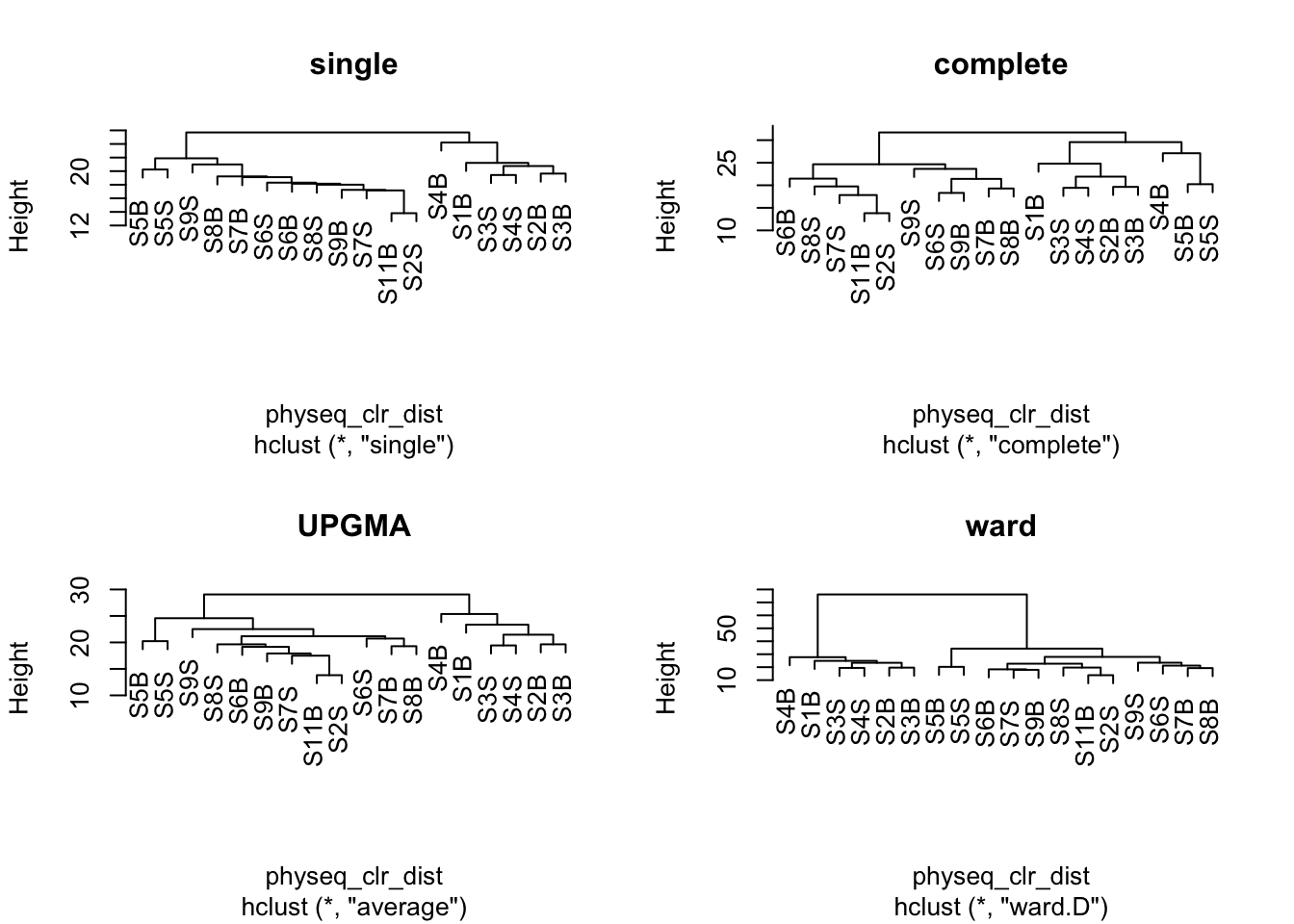
Unifrac_WU <- unifracs[, , "d_1"]physeq_clr_dist <- phyloseq::distance(physeq_clr, method = "euclidean")A first step in many microbiome projects is to examine how samples cluster on some measure of (dis)similarity. There are many ways to do perform such clustering, see here. Since microbiome data is compositional, we will perform here a hierarchical ascendant classification (HAC) of samples based on Aitchison distance.
#Simple aggregation criterion
spe_single <- hclust(physeq_clr_dist, method = "single")
#Complete aggregation criterion
spe_complete <- hclust(physeq_clr_dist, method = "complete")
#Unweighted pair group method with arithmetic mean
spe_upgma <- hclust(physeq_clr_dist, method = "average")
#Ward criterion
spe_ward <- hclust(physeq_clr_dist, method = "ward.D")

par(mfrow = c(2,2))
plot(spe_single, main = "single")
plot(spe_complete, main = "complete")
plot(spe_upgma, main = "UPGMA")
plot(spe_ward, main = "ward")
Remember that clustering is a heuristic procedure, not a statistical test. The choices of an association coefficient (similarity matrix) and a clustering method influence the result. This stresses the importance of choosing a method that is consistent with the aims of the analysis.
A cophenetic matrix is a matrix representing the cophenetic distances among all pairs of objects. A Pearson’s r correlation, called the cophenetic correlation in this context, can be computed between the original dissimilarity matrix and the cophenetic matrix. The method with the highest cophenetic correlation may be seen as the one that produced the best clustering model for the distance matrix.
Let us compute the cophenetic matrix and correlation of four clustering results presented above, by means of the function cophenetic() of package stats.
#Cophenetic correlation
spe_single_coph <- cophenetic(spe_single)
cor(physeq_clr_dist, spe_single_coph)
[1] 0.9447202spe_complete_coph <- cophenetic(spe_complete)
cor(physeq_clr_dist, spe_complete_coph)[1] 0.8609329spe_upgma_coph <- cophenetic(spe_upgma)
cor(physeq_clr_dist, spe_upgma_coph)[1] 0.958006spe_ward_coph <- cophenetic(spe_ward)
cor(physeq_clr_dist, spe_ward_coph)[1] 0.9044309Which clustering gives the most faithful representation of original distances?
To interpret and compare clustering results, users generally look for interpretable clusters. This means that a decision must be made: at what level should the dendrogram be cut? Many indices (more than 30) has been published in the literature for finding the right number of clusters in a dataset. The process has been covered here. The fusion level values of a dendrogram are the dissimilarity values where a fusion between two branches of a dendrogram occurs. Plotting the fusion level values may help define cutting levels. Let us plot the fusion level values for for the UPGMA dendrogram.
We’ll use the package NbClust which will compute, with a single function call, 24 indices for confirming the right number of clusters in the dataset:
factoextra::fviz_nbclust(t(physeq_clr@otu_table), FUNcluster =hcut, method = "silhouette", hc_method = "average", hc_metric = "euclidean", stand = TRUE)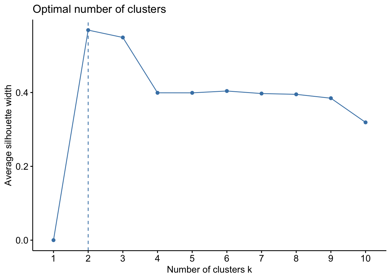
There are several ways to measure the robustness of the partitioning. Three commonly used metrics are the Dunn index, Davis-Bouldin index and Silhouette index. The Dunn index is calculated as a ratio of the smallest inter-cluster distance to the largest intra-cluster distance (good DI when you maximize InterC distance, minimize IntraC distance) . A high DI means better partionning since observations in each cluster are closer together, while clusters themselves are further away from each other. We’ll use the function cluster.stats() in fpc package for computing the Dunn index which can be used for cluster validation,
#Apply the clustering with 2 clusters
spe_upgma_clust <- cutree(tree = spe_upgma, k = 2)
#test the robustness
cs <- fpc::cluster.stats(d = physeq_clr_dist,
                         clustering = spe_upgma_clust)

cs$dunn
[1] 0.9231545The Dunn index is high indicating a good clustering of samples. Now that we identified two groups of samples based on their microbial community composition, we may want to look at which microbial clades or ASVs are enriched in each of the groups. Change the option k to see if you have a better score with more clusters…
#label are stored here for dendogram
spe_upgma$labels
[1] "S11B" "S1B" "S2B" "S2S" "S3B" "S3S" "S4B" "S4S" "S5B" "S5S"
[11] "S6B" "S6S" "S7B" "S7S" "S8B" "S8S" "S9B" "S9S" #Change with label with Description column of physeq@sam_data (because they are in same order)
spe_upgma$labels<-physeq@sam_data$Description
#apply
factoextra::fviz_dend(spe_upgma, k = 2, # Cut in four groups
cex = 0.4, # label size
color_labels_by_k = FALSE, # color labels by groups
palette = "jco", # Color palette see
rect = TRUE, rect_fill = TRUE,
rect_border = "jco", # Rectangle color
labels_track_height = 0,
)Warning: The `<scale>` argument of `guides()` cannot be `FALSE`. Use "none" instead as
of ggplot2 3.3.4.
ℹ The deprecated feature was likely used in the factoextra package.
Please report the issue at <https://github.com/kassambara/factoextra/issues>.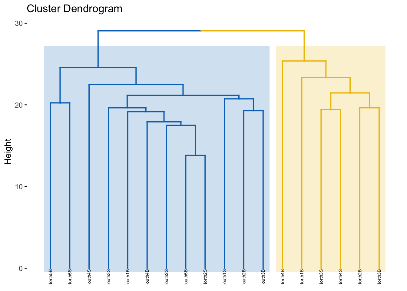
Do the groups obtained make sense?
Z-score heatmap are normalized (centered around the mean (by line!!) & reduced (Standard deviation= SD). It’s the comparison on an observed value of a sample to the mean of the population. So, it answers to the question, how far from the population mean is a score for a given sample. The scores are given in SD to the population mean.
Here we used ASV but of course you can do it on Family or genus taxonomic level!
#Transform Row/normalized counts in percentage: transform_sample_counts
pourcentS <- phyloseq::transform_sample_counts(physeq_rar, function(x) x/sum(x) * 100)
#Selection of top 30 taxa
mytop30 <- names(sort(phyloseq::taxa_sums(pourcentS), TRUE)[1:30])
#Extraction of taxa from the object pourcentS
selection30 <- phyloseq::prune_taxa(mytop30, pourcentS)
#See new object with only the top 30 ASV
selection30
phyloseq-class experiment-level object
otu_table() OTU Table: [ 30 taxa and 18 samples ]
sample_data() Sample Data: [ 18 samples by 21 sample variables ]
tax_table() Taxonomy Table: [ 30 taxa by 7 taxonomic ranks ]
phy_tree() Phylogenetic Tree: [ 30 tips and 29 internal nodes ]
refseq() DNAStringSet: [ 30 reference sequences ]#Retrieve abundance of ASV (otu_table) as table & put in data.prop variable
selection30_asv <- phyloseq::otu_table(selection30)
selection30_sample <- phyloseq::sample_data(selection30)
#Change the rownames
#See
rownames(selection30_asv) [1] "S11B" "S1B" "S2B" "S2S" "S3B" "S3S" "S4B" "S4S" "S5B" "S5S"
[11] "S6B" "S6S" "S7B" "S7S" "S8B" "S8S" "S9B" "S9S" #Change...
sample_new_names <- paste(rownames(selection30_asv),
selection30_sample$Description,
sep = "_")
#apply change
rownames(selection30_asv) <-sample_new_names
#Z-score transformation (with scale)
heat <- t(base::scale(selection30_asv))
#See
head(data.frame(heat)) S11B_South5B S1B_North1B S2B_North2B S2S_North2S S3B_North3B S3S_North3S
ASV1 0.3094323 0.3094323 -0.90630676 0.337705293 -0.6518498 -0.3408467
ASV2 -0.4230187 -0.6458135 -0.64581346 0.310893289 -0.6458135 -0.4492299
ASV3 0.9933032 -1.3409593 -0.79464254 0.993303171 -0.9436380 -2.1356018
ASV4 0.6566858 -1.1706138 -0.54247956 -0.942201337 -1.1706138 -0.7994436
ASV5 1.3481348 0.7225417 0.06402269 1.743246284 0.1298746 -0.1006071
ASV6 -0.2051885 0.4390079 0.61079364 0.009543651 2.5004365 -1.4506349
S4B_North4B S4S_North4S S5B_North5B S5S_North5S S6B_South1B S6S_South1S
ASV1 -1.811042802 -0.4256657 1.80790136 2.3450884 1.1010763 -0.1146627
ASV2 -0.580285600 -0.5933912 -0.43612431 -0.6458135 0.2846821 3.5610751
ASV3 0.099330317 -0.6456471 -0.04966516 -0.6456471 0.5959819 -0.6456471
ASV4 -0.314067112 -1.1706138 1.62743867 1.3133716 -0.6852373 -0.7423404
ASV5 0.195726498 0.3274303 -1.28594138 -0.1335330 1.0847272 -1.2859414
ASV6 0.009543651 -1.4506349 -0.07634921 -1.4506349 -0.3769742 -0.8064385
S7B_South2B S7S_South2S S8B_South3B S8S_South3S S9B_South4B S9S_South4S
ASV1 -0.82148776 -0.14293573 -0.8780338 -0.5387577 0.08324828 0.33770529
ASV2 0.78269388 -0.09537944 0.3895267 -0.5540745 0.36331558 0.02257071
ASV3 0.04966516 0.44698643 1.0429683 1.8872760 0.34765611 0.74497738
ASV4 0.91364978 1.37047467 0.8850982 0.9707529 0.48537645 -0.68523734
ASV5 -1.28594138 -1.28594138 -1.2859414 0.1957265 1.31520890 -0.46279256
ASV6 -0.41992063 0.48195436 0.7825794 0.2242758 -0.20518849 1.38382935ComplexHeatmap::Heatmap(
heat,
row_names_gp = grid::gpar(fontsize = 6),
cluster_columns = FALSE,
heatmap_legend_param = list(direction = "vertical",
title = "Z-scores",
grid_width = unit(0.5, "cm"),
legend_height = unit(3, "cm"))
)
#get taxnomic table
taxon <- as.data.frame(phyloseq::tax_table(selection30))

#concatene ASV with Phylum & Family names
myname <- paste(rownames(taxon), taxon$Phylum, taxon$Family, sep="_")
#apply
colnames(selection30_asv) <- myname#re-run Z-score to take into account the colnames change
heat <- t(scale(selection30_asv))
my_top_annotation <- ComplexHeatmap::anno_block(gp = grid::gpar(fill =c(3,4)),
labels = c(1, 2),
labels_gp = grid::gpar(col = "white",
fontsize = 10))
ComplexHeatmap::Heatmap(
heat,
row_names_gp = grid::gpar(fontsize = 6),
cluster_columns =TRUE,
heatmap_legend_param = list(direction = "vertical",
title ="Z-scores",
grid_width = unit(0.5, "cm"),
legend_height = unit(4, "cm")),
top_annotation = ComplexHeatmap::HeatmapAnnotation(foo = my_top_annotation),
column_km = 2,
column_names_gp= grid::gpar(fontsize = 6)
)
boxplot <- ComplexHeatmap::anno_boxplot(t(selection30_asv),
                                        which = "row",
                                        gp = grid::gpar(fill = "turquoise3"))

my_boxplot_left_anno <- ComplexHeatmap::HeatmapAnnotation(Abund = boxplot,
                                                          which = "row",
                                                          width = unit(3, "cm"))

my_top_anno <- ComplexHeatmap::anno_block(gp = grid::gpar(fill = c(3, 6)),
                                          labels = c("South", "North"),
                                          labels_gp = grid::gpar(col = "white",
                                                                fontsize = 10))

my_top_anno <- ComplexHeatmap::HeatmapAnnotation(foo = my_top_anno)

ComplexHeatmap::Heatmap(
  heat,
  row_names_gp = grid::gpar(fontsize = 7),
  left_annotation = my_boxplot_left_anno,
  heatmap_legend_param = list(direction = "vertical",
                              title ="Z-scores",
                              grid_width = unit(0.5, "cm"),
                              legend_height = unit(3, "cm")),
  top_annotation = my_top_anno,
  column_km = 2,
  cluster_columns = TRUE,
  column_dend_side = "bottom",
  column_names_gp = grid::gpar(fontsize = 7)
  )
We can now observe that microbial communities in samples from the south differ in their microbial composition from sample from the north. The significant effect of treatment (North/south) remains to be tested statistically, we’ll see how it is done in the hypothese testing section. This difference in community composition is due to the apparent differential abundance of many top ASV of the dataset. The identification of significant biomarkers in North and South samples will be covered in the differential abundance testing section.
While cluster analysis looks for discontinuities in a dataset, ordination extracts the main trends in the form of continuous axes. It is therefore particularly well adapted to analyse data from natural ecological communities, which are generally structured in gradients. That is why these type of analysis are called gradient analysis. The aim of ordination methods is to represent the data along a reduced number of orthogonal axes, constructed in such a way that they represent, in decreasing order, the main trends of the data. We’ll see four types of analysis widely used in ecology: PCA, PCoA, NMDS. All these methods are descriptive: no statistical test is provided to assess the significance of the structures detected. That is the role of constrained ordination or hypothese testing analysis that are presented in the following chapters.
Principal components analysis (PCA) is a method to summarise, in a low-dimensional space, the variance in a multivariate scatter of points. In doing so, it provides an overview of linear relationships between your objects and variables. This can often act as a good starting point in multivariate data analysis by allowing you to note trends, groupings, key variables, and potential outliers. Again, because of the compositional nature of microbiome data, we will use the Aitchinson distance here. Be aware that this is the CLR transformed ASV table which is used directly not the Aitchinson distance matrix. The function will calculate a euclidean distance on this CLR transformed table to get the Aitchison matrix. There are many packages allowing PCA analysis. We will use the recent PCAtools package wich provides functions for data exploration via PCA, and allows the user to generate publication-ready figures.
First, we will use a scree plot to examine the proportion of total variation explained by each PC.
#prepare the ASV table to add taxonomy
tax_CLR <-  as.data.frame(phyloseq::tax_table(physeq_clr)) #get taxnomic table
#prepare ASV table
table_clr_asv<-data.frame(t(physeq_clr@otu_table))

#concatene ASV with Family & Genus names
ASVname <- paste(rownames(tax_CLR), tax_CLR$Family, tax_CLR$Genus,sep="_")
#apply
rownames(table_clr_asv) <- ASVname

p <- PCAtools::pca(table_clr_asv,
                   metadata = data.frame(sample_data(physeq_clr)))
PCAtools::screeplot(p, axisLabSize = 18, titleLabSize = 22)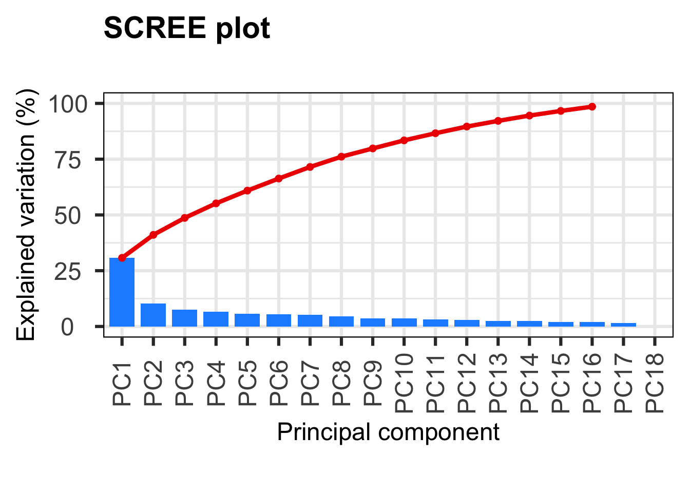
#variance explained by each PC
p$variance
PC1 PC2 PC3 PC4 PC5 PC6
3.075855e+01 1.031496e+01 7.599351e+00 6.503439e+00 5.730059e+00 5.408493e+00
PC7 PC8 PC9 PC10 PC11 PC12
5.190984e+00 4.610939e+00 3.688116e+00 3.619816e+00 3.196232e+00 2.988529e+00
PC13 PC14 PC15 PC16 PC17 PC18
2.558172e+00 2.373339e+00 2.088026e+00 1.905741e+00 1.465248e+00 2.292797e-30 Here we see that the first PC really stands out with 31% of the variance explained and then we have a gradual decline for the remaining components. A scree plot on its own just shows the accumulative proportion of explained variation, but we want to determine the optimum number of PCs to retain (SEE ANF practice).
PCAtools::pairsplot(p)
#Plotting the PCA
PCAtools::biplot(
  p,
  lab = p$metadata$Description,
  colby = "Geo",
  pointSize = 5,
  hline = 0, vline = 0,
  legendPosition = "right"
)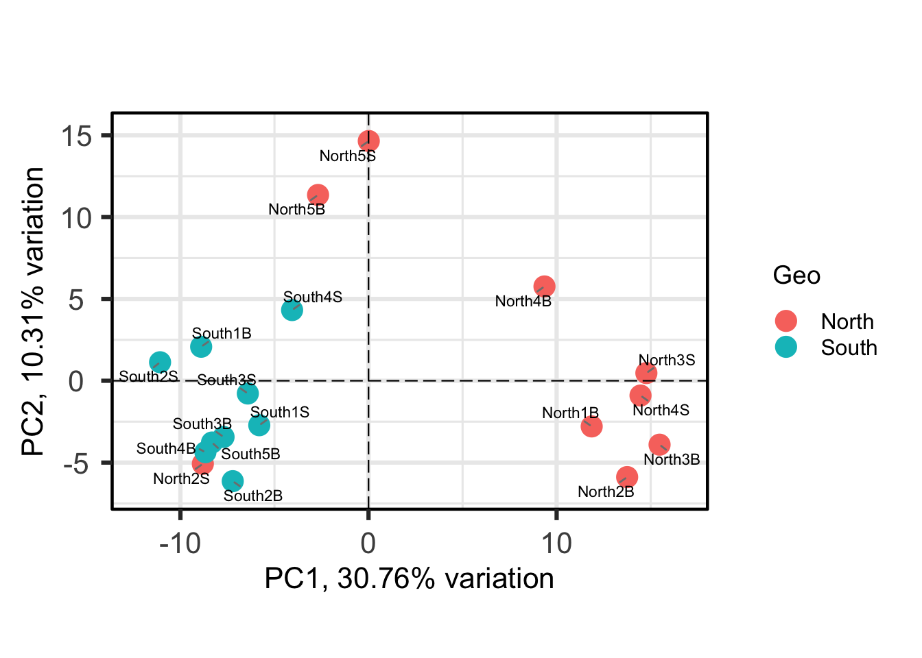
Each point is a sample, and samples that appear closer together are typically more similar to each other than samples which are further apart. So by colouring the points by treatment you can see that the microbiota from the North are often, but not always, highly distinct from sample from the south.
One benefit of not using a distance matrix, is that you can plot taxa “loadings” onto your PCA axes, using the showLoadings = TRUE argument. PCAtools allow you to plots the number of taxa loading vectors you want beginning by those having the more weight on each PCs. The relative length of each loading vector indicates its contribution to each PCA axis shown, and allows you to roughly estimate which samples will contain more of that taxon. https://www.bioconductor.org/packages/devel/bioc/vignettes/PCAtools/inst/doc/PCAtools.html
bp <- PCAtools::biplot(
  p,
  showLoadings = TRUE,
  boxedLoadingsNames = FALSE,
  lengthLoadingsArrowsFactor = 1.5,
  sizeLoadingsNames = 3,
  colLoadingsNames = 'red4',
  ntopLoadings = 3,
  colby = "Geo",
  hline = 0, vline = 0,
  legendPosition = "right"
)
bp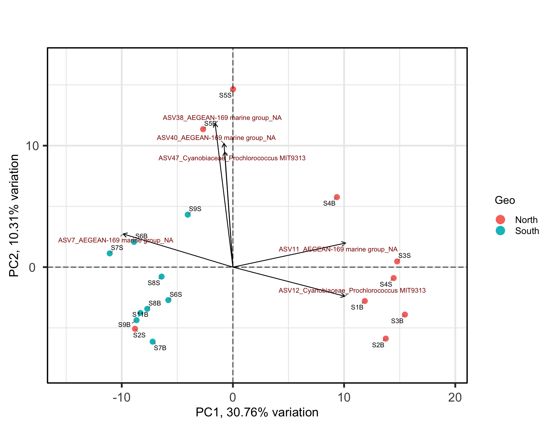
ASVs 7, 11 and 12 have a high contribution to PC1 while ASVs 40, 38, and 47 have a high contribution on the second PC. These ASVs belong to only two families. Samples from the South seems to be enriched in ASV7 while North samples contain higher abundances of ASV11 and 12. The two Noth sample outliers at the top of the plot are caracterized by a higher abundance of ASVs 40, 38, and 47.
#Select variable of interest in your sam_data
env<- data.frame(physeq@sam_data[,c(11:15,19:21)])
#use envfit function

set.seed(123)  # Fixer
env_fit <- vegan::envfit(p$rotated, env, permutations = 999)
# Extraire les scores des vecteurs environnementaux à partir de l'objet env_fit
env_scores <- as.data.frame(vegan::scores(env_fit, display = "vectors"))
# Sélectionner les vecteurs significatifs (p-value < 0.05)
significant <- env_fit$vectors$pvals < 0.05
# garder que les significants
env_data <- env_scores[significant, , drop = FALSE]
#stocker les noms
env_data$var <- rownames(env_data) # ajouter le nom de la variablebp +
geom_segment(data = env_data,
aes(x = 0, y = 0,
xend = PC1 * 10, yend = PC2 * 10),
arrow = arrow(length = unit(0.1, "inches")),
color = "blue") +
geom_text(data = env_data,
aes(x = PC1 * 10, y = PC2 * 10, label = var),
color = "blue", vjust = -0.5)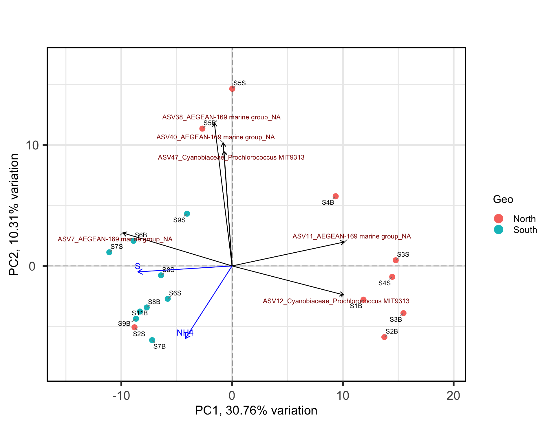
Significant correlation found between the first PC1 explaining the separation between South and North samples are salinity and to a lesser extend NH4. This is interesting but correlation between variables does not automatically means that the change in one variable is the cause of the change in the values of the other variable. We’ll check later if there is a causal relationship between the salinity gradient and the difference observed in southern and northern bacterial communities.
Principal coordinates analysis (PCoA, also known as metric multidimensional scaling, MDS) attempts to represent the distances between samples in a low-dimensional, Euclidean space. In particular, it maximizes the linear correlation between the distances in the distance matrix, and the distances in a space of low dimension (typically, 2 or 3 axes are selected). As always, the choice of (dis)similarity measure is critical and must be suitable to the data in question. Here we will use the Bray-Curtis distance. When the distance metric is Euclidean, PCoA is equivalent to Principal Components Analysis. The interpretation of the results is the same as with PCA.
#PCoA on Bray-Curtis dissimilarity
physeq_rar_bray=ordinate(physeq_rar,"MDS",distance = "bray")
PcoA=plot_ordination(physeq_rar,physeq_rar_bray, type="samples", color="Geo")+ geom_text(mapping = aes(label = Description), size = 2,vjust = 2.1)
PcoA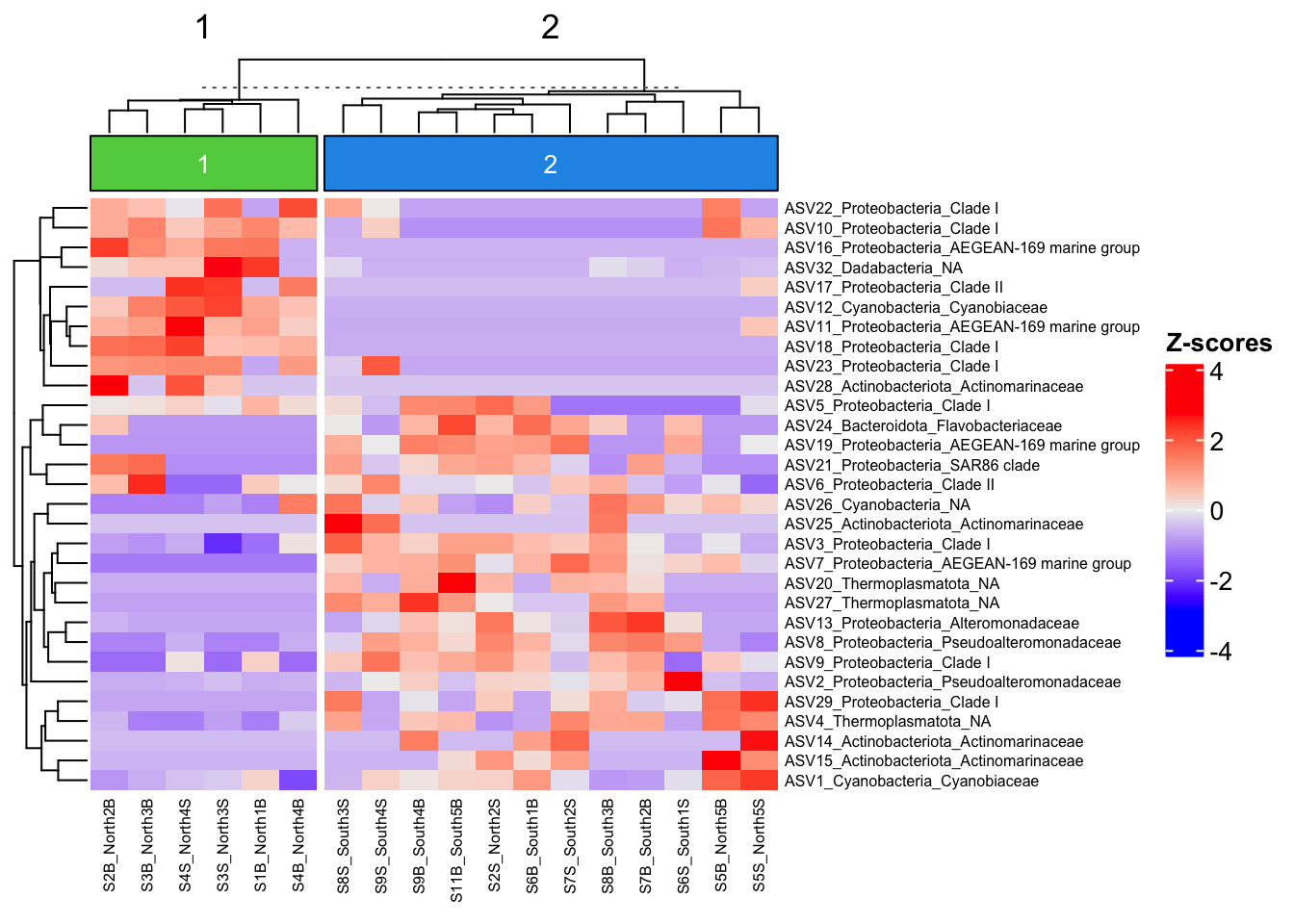
The ordination of the samples in the PCoA is very similar to the one observed in the PCA with a clear segregation of North and South bacterial communities. This segregation may result from the increasing salinity gradient from North to South but it relaims to be tested.
Do you see what is missing?
Indeed, there are no species plotted on this ordination. That’s because we used a dissimilarity matrix (sites x sites) as input for the PCoA function. Hence, no species scores could be calculated. However, we could work around this problem with the function biplot.pcoa() from the ape package or with plot_ordination from phyloseq (split or biplot).
Split option separate in two box the site and the ASV/species, but it can be drawn on same plot.
Unif= plot_ordination(physeq_rar,physeq_rar_bray, type="split", color="Phylum")+ geom_text(mapping = aes(label = Description), size = 2,vjust = 2.1)
Unif
Warning: Removed 209 rows containing missing values or values outside the scale range
(`geom_text()`).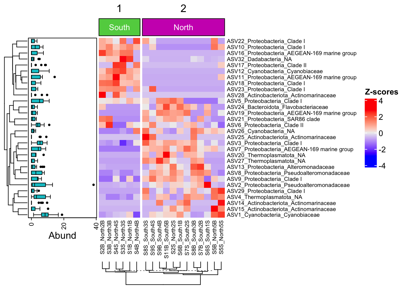
PCoA suffers from a number of flaws, in particular the arch effect (see PCA for more information). These flaws stem, in part, from the fact that PCoA maximizes a linear correlation. Non-metric Multidimensional Scaling (NMDS) rectifies this by maximizing the rank order correlation.
set.seed(123)  # Fixer
env_fitPcoA <- vegan::envfit(physeq_rar_bray$vectors, env, permutations = 999)
# Extraire les scores des vecteurs environnementaux à partir de l'objet env_fit
env_scoresPcoA <- as.data.frame(vegan::scores(env_fitPcoA, display = "vectors"))
# Sélectionner les vecteurs significatifs (p-value < 0.05)
significantPcoA <- env_fitPcoA$vectors$pvals < 0.05
# garder que les significants
env_dataPcoA <- env_scoresPcoA[significantPcoA, , drop = FALSE]
#stocker les noms
env_dataPcoA$var <- rownames(env_dataPcoA)  # ajouter le nom de la variable
PcoA +
geom_segment(data = env_dataPcoA,
aes(x = 0, y = 0,
xend = Axis.1, yend = Axis.2),
arrow = arrow(length = unit(0.1, "inches")),
color = "blue") +
geom_text(data = env_dataPcoA,
aes(x = Axis.1, y = Axis.2, label = var),
color = "blue", vjust = -0.5)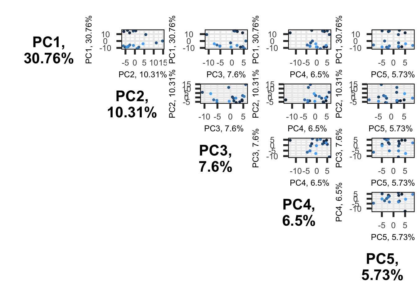
NMDS attempts to represent the pairwise dissimilarity between objects in a low-dimensional space. Any dissimilarity coefficient or distance measure may be used to build the distance matrix used as input. NMDS is a rank-based approach. This means that the original distance data is substituted with ranks. While information about the magnitude of distances is lost, rank-based methods are generally more robust to data which do not have an identifiable distribution.
NMDS is an iterative algorithm. NMDS routines often begin by random placement of data objects in ordination space. The algorithm then begins to refine this placement by an iterative process, attempting to find an ordination in which ordinated object distances closely match the order of object dissimilarities in the original distance matrix. The stress value reflects how well the ordination summarizes the observed distances among the samples.
NMDS is not an eigenanalysis. This has three important consequences:
Axes are not ordered in NMDS. vegan::metaMDS() automatically rotates the final result of the NMDS using PCA to make axis 1 correspond to the greatest variance among the NMDS sample points.
#NMDS plot
physeq_nmds <- vegan::metaMDS(physeq_rar@otu_table, k=2, trymax=100, distance = "bray")
Square root transformation
Wisconsin double standardization
Run 0 stress 0.09103176
Run 1 stress 0.09103177
... Procrustes: rmse 4.17487e-06 max resid 1.396203e-05
... Similar to previous best
Run 2 stress 0.09103166
... New best solution
... Procrustes: rmse 0.0001305564 max resid 0.000455967
... Similar to previous best
Run 3 stress 0.09103165
... New best solution
... Procrustes: rmse 0.0001254305 max resid 0.0004383245
... Similar to previous best
Run 4 stress 0.1222939
Run 5 stress 0.1061511
Run 6 stress 0.1208745
Run 7 stress 0.1061511
Run 8 stress 0.09103172
... Procrustes: rmse 0.0001219846 max resid 0.000424785
... Similar to previous best
Run 9 stress 0.09103171
... Procrustes: rmse 0.0001044806 max resid 0.0003613363
... Similar to previous best
Run 10 stress 0.1125521
Run 11 stress 0.09103183
... Procrustes: rmse 0.0003073399 max resid 0.00107377
... Similar to previous best
Run 12 stress 0.09474918
Run 13 stress 0.09103167
... Procrustes: rmse 5.039975e-05 max resid 0.0001750975
... Similar to previous best
Run 14 stress 0.09103167
... Procrustes: rmse 5.990951e-05 max resid 0.0002079029
... Similar to previous best
Run 15 stress 0.09433861
Run 16 stress 0.09103176
... Procrustes: rmse 0.0001625622 max resid 0.0005665919
... Similar to previous best
Run 17 stress 0.09474927
Run 18 stress 0.1125521
Run 19 stress 0.1061511
Run 20 stress 0.1061511
*** Best solution repeated 7 timesA useful way to assess the appropriateness of an NMDS result is to compare, in a Shepard diagram, the distances among objects in the ordination plot with the original distances.
#See stress
physeq_nmds$stress
[1] 0.09103165#Plot correlation ordination distance vs. dissimilarities in matrix
vegan::stressplot(physeq_nmds)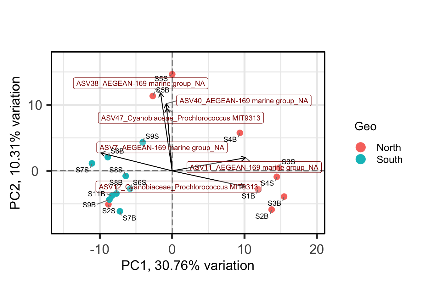
There is a good non-metric fit between observed dissimilarities (in our distance matrix) and the distances in ordination space. Also the stress of our final result was good.
do you know how much the stress is?
The stress value can be used as an indicator of the goodness-of-fit. Stress values >0.2 are generally poor and potentially not interpretable, whereas values <0.1 are good and <0.05 are excellent, leaving little danger of misinterpretation.
So we can go further and plot the results:
#Sites
data.scores = as.data.frame(vegan::scores(physeq_nmds)$sites)
#Add column with group info North-South contained in Geo of sample_data
data.scores$groupe= physeq_rar@sam_data$Geo
#See
data.scores
NMDS1 NMDS2 groupe
S11B -0.4641189 -0.09931835 South
S1B 0.9408343 -0.64295956 North
S2B 0.9302240 -0.10684574 North
S2S -0.4943642 -0.12352357 North
S3B 1.1432453 -0.22472717 North
S3S 1.1103814 0.11334785 North
S4B 0.7047197 0.62393568 North
S4S 0.9947323 0.06898251 North
S5B -0.3121428 0.50911321 North
S5S -0.2298842 0.59582519 North
S6B -0.5602960 0.15136813 South
S6S -0.9917779 -0.22954834 South
S7B -0.4866566 -0.46113247 South
S7S -0.5567694 0.04381655 South
S8B -0.5256230 -0.26247413 South
S8S -0.3850055 -0.01126064 South
S9B -0.5755250 -0.13195849 South
S9S -0.2419737 0.18735933 South#Species
data.scoressp = as.data.frame(vegan::scores(physeq_nmds)$species)
#PlotNMDS=ggplot()+
geom_point(data=data.scores, aes(x = NMDS1, y = NMDS2, colour=groupe), size = 3, alpha = 0.5)+
geom_text(data=data.scores, size= 2,hjust=-0.4, vjust=0.6, aes(x = NMDS1, y = NMDS2,label=rownames(data.scores)))+
scale_colour_manual(values = c("orange", "steelblue"))+
geom_point(data=data.scoressp, aes(x = NMDS1, y = NMDS2),shape=3, size = 1, colour="red")
PlotNMDS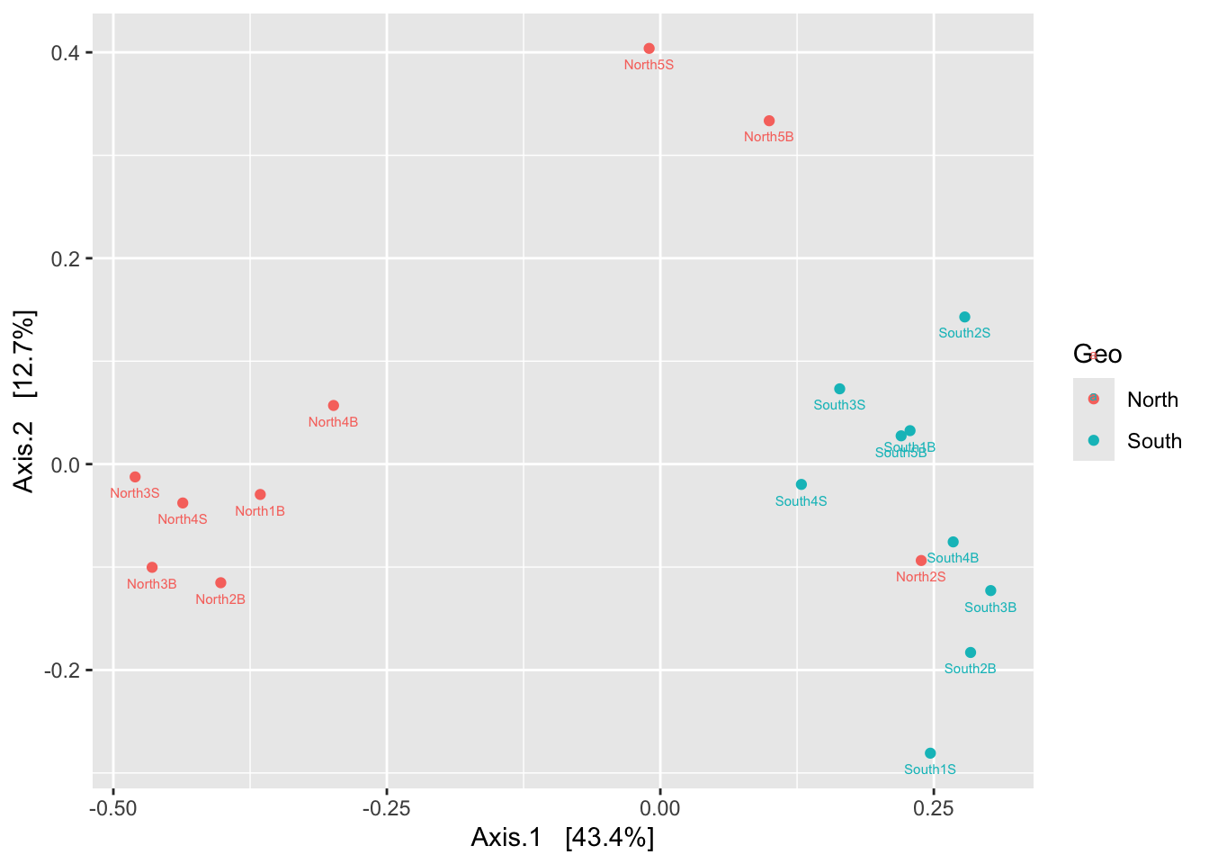
The next question is: Which environmental variable is driving the observed differences in species composition? Similarly to what we have done with PCA, we can correlate environmental variables with our ordination axes.
set.seed(123)  # Fixer
env_fitNMDS <- vegan::envfit(physeq_nmds, env, permutations = 999)
env_fitNMDS
***VECTORS

           NMDS1    NMDS2     r2 Pr(>r)
SiOH4   -0.89645 -0.44315 0.3001  0.077 .
NO2     -0.50059 -0.86569 0.3690  0.040 *
NO3      0.80783  0.58942 0.2739  0.097 .
NH4     -0.57604 -0.81742 0.4778  0.008 **
PO4     -0.82169 -0.56993 0.2806  0.088 .
T       -0.85040 -0.52613 0.2798  0.093 .
S       -0.95592 -0.29363 0.7604  0.001 ***
Sigma_t -0.99621 -0.08692 0.2523  0.124
---
Signif. codes:  0 '***' 0.001 '**' 0.01 '*' 0.05 '.' 0.1 ' ' 1
Permutation: free
Number of permutations: 999
# Extraire les scores des vecteurs environnementaux à partir de l'objet env_fit
env_scoresNMDS <- as.data.frame(vegan::scores(env_fitNMDS, display = "vectors"))
# Sélectionner les vecteurs significatifs (p-value < 0.05)
significantNMDS <- env_fitNMDS$vectors$pvals < 0.05
# garder que les significants
env_dataNMDS <- env_scoresPcoA[significantNMDS, , drop = FALSE]
env_dataNMDS Axis.1 Axis.2
NO2 0.3873443 -0.34516824
NH4 0.4017809 -0.64915059
S 0.8651446 -0.05273686#stocker les noms
env_dataNMDS$var <- rownames(env_dataNMDS) # ajouter le nom de la variablePlotNMDS +
geom_segment(data = env_dataNMDS,
aes(x = 0, y = 0,
xend = Axis.1, yend = Axis.2),
arrow = arrow(length = unit(0.1, "inches")),
color = "blue") +
geom_text(data = env_dataNMDS,
aes(x = Axis.1, y = Axis.2, label = var),
color = "blue", vjust = -0.5)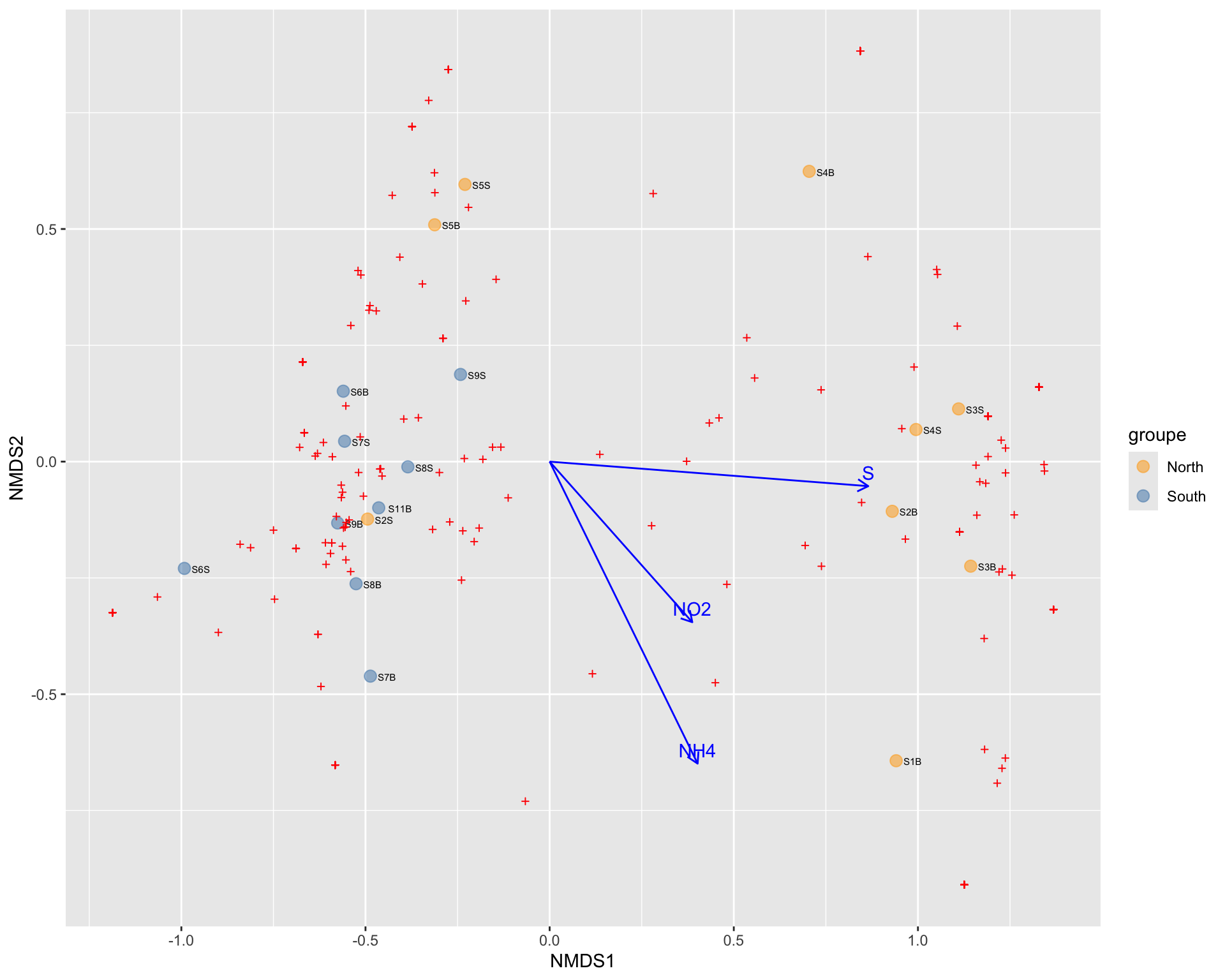
Here again, we can see that the salinity is strongly correlated with the first axis separating samples from the South and the North. To a lesser extent, new environmental variables related with the trophic conditions of the habitat (NH4 and NO2) were correlated with the second axis of the NMDS. The detection of these new relations between microbial communities and the environment may be related to the fact that NMDS is best suited to detect the non linear response of microbes to environmental gradients.
Many different types of indirect gradient analysis are available out there. In the following graph, we offer suggestions of some of the appropriate choices based on data input structure and expected relationships among variables.
We saw some segregation between Northern and Southern samples suggesting some differences in the bacterial communities according to sample type. While indirect gradient or classification analyses are exploratory data visualization tool, we can test whether the samples cluster beyond that expected using hypotheses testing methods such as multivariate analysis of variance with permutation (PERMANOVA), and analysis of group similarities (ANOSIM), multi-response permutation procedures (MRPP), and Mantel’s test (MANTEL) and more recently Dirichlet-multinomial models.
PERMANOVA was proposed by Anderson and McArdle to apply the powerful ANOVA to multivariate ecological datasets. PERMANOVA is one of most widely used nonparametric methods to fit multivariate models to microbiome data. It is a multivariate analysis of variance based on distance matrices and permutation. It does this by partitioning the sums of squares for the within- and between-cluster components using the concept of centroids. Many permutations of the data (i.e. random shuffling) are used to generate the null distribution. Find more informations on PERMANOVA here and on the adonis2() function here Now let us evaluate whether the group (North vs. South) has a significant effect on overall bacterial community composition. PERMANOVA is insensitive to many zero, you need balanced groups.
#PERMANOVA
metadata <- data.frame(phyloseq::sample_data(physeq_clr))
results_permanova <- vegan::adonis2(physeq_clr_dist ~ Geo,
                                    data = metadata,
                                    perm = 1000)
results_permanova
Permutation test for adonis under reduced model
Terms added sequentially (first to last)
Permutation: free
Number of permutations: 1000
vegan::adonis2(formula = physeq_clr_dist ~ Geo, data = metadata, permutations = 1000)
Df SumOfSqs R2 F Pr(>F)
Geo 1 1135.5 0.20329 4.0825 0.000999 ***
Residual 16 4450.1 0.79671
Total 17 5585.6 1.00000
---
Signif. codes: 0 '***' 0.001 '**' 0.01 '*' 0.05 '.' 0.1 ' ' 1Here we can see that the North/South grouping explain significantly (p < 0.001) 20% of the variance in the ASV bray matrix. In other words Northern and Southern bacterial differ significantly in their bacterial composition. The test from ADONIS can be confounded by differences in dispersion (or spread) so we want to check this as well.. You want to show that your groups have different centroid or not… but dispersion can biais the primary result of PERMANOVA.
# Testing the assumption of similar multivariate spread among the groups (ie. analogous to variance homogeneity)
anova(vegan::betadisper(physeq_clr_dist, metadata$Geo))
Analysis of Variance Table
Response: Distances
Df Sum Sq Mean Sq F value Pr(>F)
Groups 1 49.657 49.657 13.915 0.001822 **
Residuals 16 57.096 3.569
---
Signif. codes: 0 '***' 0.001 '**' 0.01 '*' 0.05 '.' 0.1 ' ' 1dispersion=vegan::betadisper(physeq_clr_dist, metadata$Geo)
plot(dispersion, ellipse = TRUE, hull = FALSE) 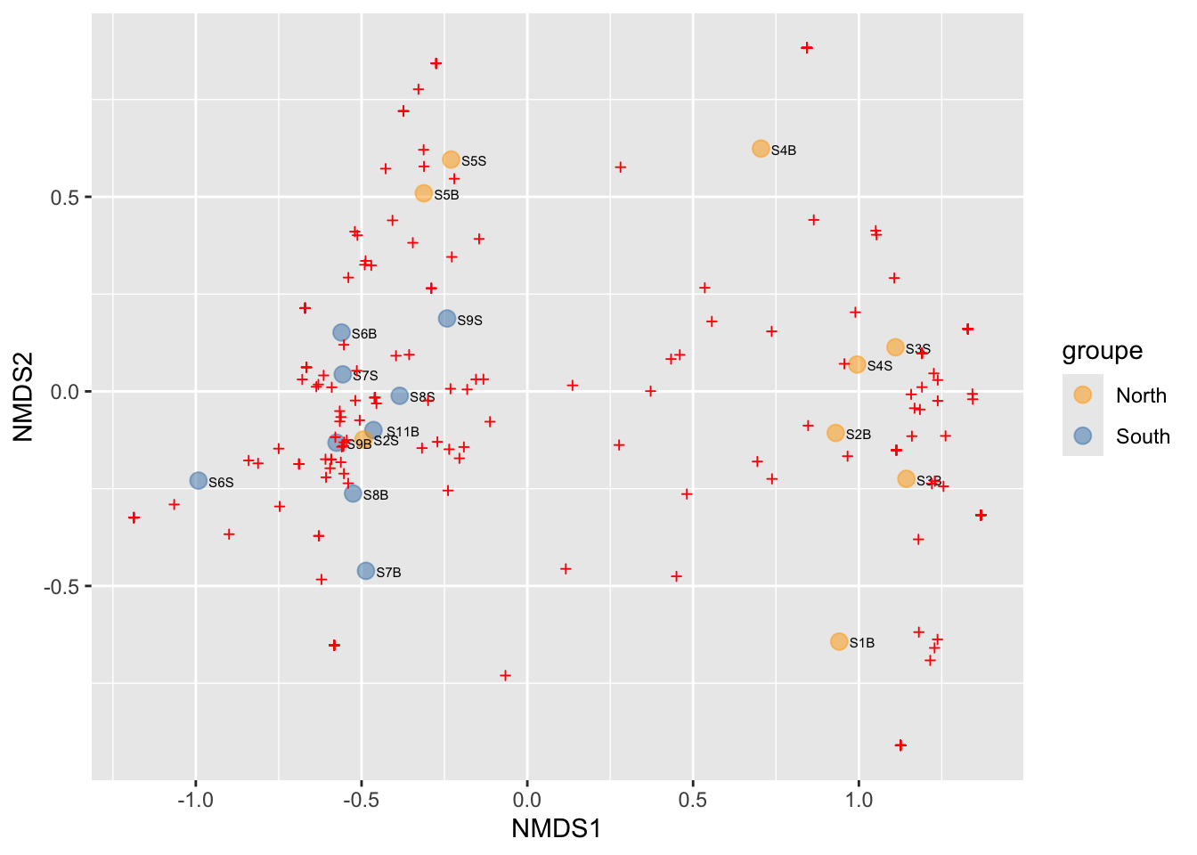
Here the groups have significant different spreads and permanova result may be impacted by that although PERMANOVA is very robust to difference in group dispersion.
adonis() and adonis2() allow us to explore the effect of categorical or continuous variables.
SEE complement here (for you at home) : ANF https://anf-metabiodiv.github.io/course-material/practicals/beta_diversity.html
Simple (unconstrained) ordination analyses one data matrix and reveals its major structure in a graph constructed from a reduced set of orthogonal axes. It is therefore a passive form of analysis, and the user interprets the ordination results a posteriori. On the contrary, direct gradient analyses (called also canonical ordination) associates two or more data sets in the ordination process itself. Consequently, if one wishes to extract structures of a data set that are related to structures in other data sets, and/or formally test statistical hypotheses about the significance of these relationships, canonical ordination is the way to go. Here we will perform a RDA on our dataset but many other types exit: distance-based redundancy analysis (db-RDA), canonical correspondence analysis (CCA), linear discriminant analysis (LDA), canonical correlation analysis (CCorA), co-inertia analysis (CoIA) and multiple factor analysis (MFA). For more informations see this excellent book.
RDA is a method combining regression and principal component analysis (PCA). RDA computes axes that are linear combinations of the explanatory variables. In RDA, one can truly say that the axes explain or model (in the statistical sense) the variation of the dependent matrix.
# RDA of the Aitchinson distance
# constrained by all the environmental variables
# contained in metadata
#
# Observe the shortcut formula
spe_rda <- vegan::rda(t(table_clr_asv) ~ .,
                      metadata[, 11:21])
head(summary(spe_rda))
Call:
rda(formula = t(table_clr_asv) ~ SiOH4 + NO2 + NO3 + NH4 + PO4 +      NT + PT + Chla + T + S + Sigma_t, data = metadata[, 11:21])

Partitioning of variance:
              Inertia Proportion
Total          328.56     1.0000
Constrained    231.46     0.7044
Unconstrained   97.11     0.2956

Eigenvalues, and their contribution to the variance

Importance of components:
                         RDA1     RDA2     RDA3     RDA4     RDA5     RDA6
Eigenvalue            85.2928 30.29173 20.29415 18.85659 15.83909 12.98651
Proportion Explained   0.2596  0.09219  0.06177  0.05739  0.04821  0.03952
Cumulative Proportion  0.2596  0.35179  0.41355  0.47094  0.51915  0.55868
                          RDA7     RDA8     RDA9   RDA10   RDA11      PC1
Eigenvalue            11.78027 10.97738 10.18119 7.94385 7.01222 28.88564
Proportion Explained   0.03585  0.03341  0.03099 0.02418 0.02134  0.08791
Cumulative Proportion  0.59453  0.62794  0.65893 0.68310 0.70445  0.79236
                           PC2     PC3      PC4      PC5     PC6
Eigenvalue            16.45693 16.3958 15.58129 11.19715 8.59184
Proportion Explained   0.05009  0.0499  0.04742  0.03408 0.02615
Cumulative Proportion  0.84245  0.8923  0.93977  0.97385 1.00000

Accumulated constrained eigenvalues
Importance of components:
                         RDA1    RDA2     RDA3     RDA4     RDA5     RDA6
Eigenvalue            85.2928 30.2917 20.29415 18.85659 15.83909 12.98651
Proportion Explained   0.3685  0.1309  0.08768  0.08147  0.06843  0.05611
Cumulative Proportion  0.3685  0.4994  0.58706  0.66853  0.73696  0.79307
                         RDA7     RDA8     RDA9   RDA10  RDA11
Eigenvalue            11.7803 10.97738 10.18119 7.94385 7.0122
Proportion Explained   0.0509  0.04743  0.04399 0.03432 0.0303
Cumulative Proportion  0.8440  0.89139  0.93538 0.96970 1.0000

Scaling 2 for species and site scores
* Species are scaled proportional to eigenvalues
* Sites are unscaled: weighted dispersion equal on all dimensions
* General scaling constant of scores:  8.645047


Species scores

                                                 RDA1      RDA2     RDA3
ASV1_Cyanobiaceae_Synechococcus CC9902        -0.1033  0.108773  0.04666
ASV2_Pseudoalteromonadaceae_Pseudoalteromonas -0.7807 -0.229145 -0.22860
ASV3_Clade I_Clade Ia                         -0.2568  0.002182 -0.22536
ASV4_NA_NA                                    -0.6996  0.193071  0.23547
ASV5_Clade I_Clade Ia                          0.5264 -0.195773  0.23032
ASV6_Clade II_NA                              -0.2542 -0.344583 -0.32380
....
                                                  RDA4     RDA5     RDA6
ASV1_Cyanobiaceae_Synechococcus CC9902         0.12535 -0.01552  0.06487
ASV2_Pseudoalteromonadaceae_Pseudoalteromonas -0.33352  0.13369  0.08880
ASV3_Clade I_Clade Ia                          0.04191 -0.04528 -0.11436
ASV4_NA_NA                                    -0.20648 -0.23531  0.06807
ASV5_Clade I_Clade Ia                          0.05792  0.40196 -0.22286
ASV6_Clade II_NA                               0.31352 -0.10920 -0.06137
....


Site scores (weighted sums of species scores)

       RDA1     RDA2    RDA3    RDA4     RDA5    RDA6
S11B -1.703 -1.23820  2.9437  0.2362  1.13728 -0.4405
S1B   2.565 -0.13340 -0.7868  5.7453  3.30268 -3.3657
S2B   3.022 -2.96571  0.4021  0.9802 -3.09213  0.9282
S2S  -1.731 -1.82618  2.0707  0.3281 -0.66853 -1.6638
S3B   3.624 -1.55655 -1.2829  2.0701 -2.02586  1.7347
S3S   3.165 -0.08923  2.8998 -2.0441 -0.08464  2.0314
....


Site constraints (linear combinations of constraining variables)

        RDA1    RDA2    RDA3    RDA4    RDA5    RDA6
S11B -1.2105 -0.7764  3.0649  0.2199  1.2569  0.7586
S1B   1.7387  0.3983 -0.3817  5.4943  3.2411 -2.7484
S2B   2.0536 -3.3237  0.6260  1.4897 -2.8936  0.1774
S2S   0.5936 -2.0609  1.1588  0.1736 -0.8183 -1.8069
S3B   4.1498 -1.1569 -1.6837  1.1942 -2.4216  2.5295
S3S   2.0704 -0.1285  3.6947 -1.1733  0.3885  1.8438
....


Biplot scores for constraining variables

            RDA1     RDA2     RDA3     RDA4     RDA5      RDA6
SiOH4   -0.57424 -0.21106 -0.25450 -0.25678 -0.02349 -0.213981
NO2     -0.51463 -0.10086 -0.08171  0.34294  0.35340  0.013696
NO3      0.59878  0.05632 -0.04267 -0.02065 -0.30772  0.095439
NH4     -0.63097 -0.49073 -0.01146 -0.07457  0.25646  0.259440
PO4     -0.49369 -0.05367 -0.31521  0.04459  0.19877  0.304690
NT       0.02778 -0.05873 -0.28198  0.59590  0.14825 -0.392684
PT      -0.61634 -0.27995 -0.01129  0.12013  0.07328 -0.533916
Chla    -0.47936 -0.07832 -0.06090 -0.01293 -0.11376  0.179421
T       -0.57485  0.21879  0.26190  0.53662 -0.42902  0.007286
S       -0.93622  0.00815 -0.06712  0.05543  0.04078  0.183950
Sigma_t -0.52380 -0.20293 -0.31121 -0.40702  0.43162  0.205711
The included environmental variables explain 70.44% of the variation in bacterial community composition across sites. 29.56 % of the variance is unexplained. However, we’ll see that the propotion of variance explained is much lower. The R2 from the summary measures the strength of the canonical relationship between the response variables (Y matrix, ASVs) and the explanatory variables (X matrix) by calculating the proportion of the variation of Y explained by the variables in X. However, this R2 is biased. We calculate an Adjusted R2, which also measures the strength of the relationship between Y and X, but applies a correction of the R2 to take into account the number of explanatory variables. This is the statistic that should be reported.
# Unadjusted R^2 retrieved from the rda object
R2 <- vegan::RsquareAdj(spe_rda)$r.squared
R2
[1] 0.7044457# Adjusted R^2 retrieved from the rda object
R2adj <- vegan::RsquareAdj(spe_rda)$adj.r.squared
R2adj[1] 0.1625961In reality, the proportion of variance explained dropped to 16.25 %. The numerical output shows that the first two canonical axes explain together 35.1% of the total variance of the data, the first axis alone explaining 25.9%. These are unadjusted values, however. Since R2 adj = 16.2 %, the percentages of accumulated constrained adj eigenvalues show that the first axis alone explains 0.162 * 0.368 = 0.059 or 5.9% variance. Because ecological data are generally quite noisy, one should never expect to obtain a very high value of R2 . Furthermore, the first unconstrained eigenvalue (PC1), the first unconstrained axe for the residuals, is comparatively high, which means that it does display an important residual structure of the response data that is not explain by the environmental parameters measure here.
The interpretation of the constrained ordination must be preceded by a test of statistical significance (see below). As in multiple regression, a non-significant result must not be interpreted and must be discarded.
# Global test of the RDA result
anova(spe_rda, step = 1000)
Permutation test for rda under reduced model
Permutation: free
Number of permutations: 999
Model: rda(formula = t(table_clr_asv) ~ SiOH4 + NO2 + NO3 + NH4 + PO4 + NT + PT + Chla + T + S + Sigma_t, data = metadata[, 11:21])
Df Variance F Pr(>F)
Model 11 231.456 1.3001 0.094 .
Residual 6 97.109
---
Signif. codes: 0 '***' 0.001 '**' 0.01 '*' 0.05 '.' 0.1 ' ' 1# Tests of all canonical axes
anova(spe_rda, by = "axis", step = 1000)Permutation test for rda under reduced model
Forward tests for axes
Permutation: free
Number of permutations: 999
Model: rda(formula = t(table_clr_asv) ~ SiOH4 + NO2 + NO3 + NH4 + PO4 + NT + PT + Chla + T + S + Sigma_t, data = metadata[, 11:21])
Df Variance F Pr(>F)
RDA1 1 85.293 5.2699 0.137
RDA2 1 30.292 1.8716 0.622
RDA3 1 20.294 1.2539 0.997
RDA4 1 18.857 1.1651 1.000
RDA5 1 15.839 0.9786 1.000
RDA6 1 12.987 0.8024 1.000
RDA7 1 11.780 0.7279 1.000
RDA8 1 10.977 0.6783 1.000
RDA9 1 10.181 0.6291 0.999
RDA10 1 7.944 0.4908 0.992
RDA11 1 7.012 0.4333 0.905
Residual 6 97.109 Here we can see that our full model is statistically non significant (p = 0.106), and every canonical axis resulting from the RDA are not either statistically significant (p > 0.05). This RDA model is not interpretable.
The temptation to build an ecological model using all available information (i.e., all variables) is hard to resist. Lots of time and money are exhausted gathering data and supporting information. We also hope to identify every significant variable to more accurately characterize relationships with biological relevance. Collinearity, or excessive correlation among explanatory variables, can complicate or prevent the identification of an optimal set of explanatory variables for a statistical model. Let’s take a look at which explanatory variables are correlated. The idea is to reduce the number of explanatory variables. The reasons vary: search for parsimony, rich data set but poor a priori hypotheses and possible strong linear dependencies (correlations) among the explanatory variables in the RDA model, which could render the regression coefficients of the explanatory variables in the model unstable.
ANF : correlation spearman exple. https://anf-metabiodiv.github.io/course-material/practicals/beta_diversity.html
env = metadata[,11:21]
res.pca <- FactoMineR::PCA(env,  graph = FALSE)
fviz_pca_var(res.pca, col.var = "contrib", gradient.cols = c("#00AFBB", "#E7B800", "#FC4E07"))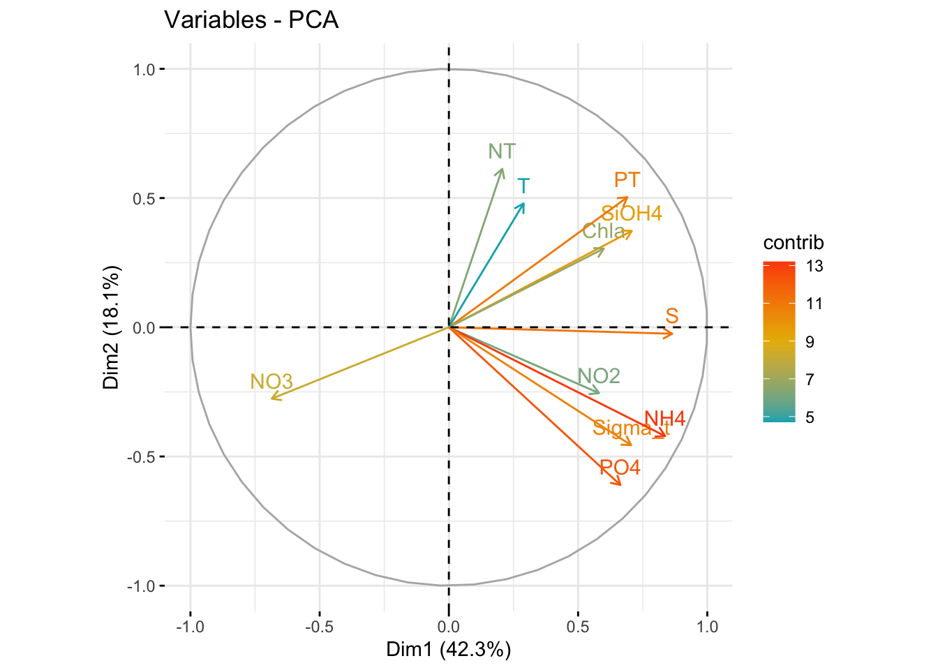
The VIF quantifies the inflation of a variable’s variance due to its collinearity with all the other variables in the model. In other words, it measures multicollinearity by taking into account the combined effect of the other variables. VIF calculations are straightforward and easily comprehensible; the higher the value, the higher the collinearity. VIF measure the proportion by which the variance of a regression coefficient is inflated in the presence of other explanatory variables. VIFs above 20 indicate strong collinearity. Ideally, VIFs above 10 should be at least examined, and avoided if possible.
# Variance inflation factors (VIF)
vegan::vif.cca(spe_rda)
SiOH4 NO2 NO3 NH4 PO4 NT
4.066588 3.489186 3.634643 16.867288 8.819736 4.908553
PT Chla T S Sigma_t
6.835572 2.264012 5417.455601 8388.550079 6878.896122 Salinity, Temperature and Sigma.t have very hight VIFs. A reduction of the number of explanatory variables is justified. In order to simplify this model, we can perform a forward selection (or backwards). These types of selections help us select variables that are statistically important. However, it is important to note that selecting variables ecologically is much more important than performing selection in this way. If a variable of ecological interest is not selected, this does not mean it has to be removed from the RDA. Here, we will be performing forward selection on our 11 environmental variables. To do this, we can use the ordiR2step() function:
# Forward selection of explanatory variables using vegan's ordiR2step()
step_forward <- vegan::ordiR2step(vegan::rda(t(table_clr_asv) ~ 1,
                                             data = metadata[,11:21]),
                                  scope = formula(spe_rda),
                                  direction = "forward",
                                  pstep = 1000)
Step: R2.adj= 0
Call: t(table_clr_asv) ~ 1
R2.adjusted
+ S 0.18366030
<All variables> 0.16259613
+ NH4 0.08392874
+ PT 0.07013415
+ T 0.06719602
+ NO3 0.05904665
+ SiOH4 0.05787026
+ Sigma_t 0.05002017
+ NO2 0.03846019
+ PO4 0.03190148
+ Chla 0.02451726
<none> 0.00000000
+ NT -0.01448677Here, we are essentially adding one variable at a time, and retaining it if it significantly increases the model’s adjusted R2. The forward selection show us that a model with only salinity has higher R2 adjust than with all variable and explain 18.4 % of the variance. Lets calculate this most parsimonious RDA and check its significance.
# Parsimonious RDA
spe_rda_pars <- vegan::rda(t(table_clr_asv) ~ S, data = env)
anova(spe_rda_pars, step = 1000)
Permutation test for rda under reduced model
Permutation: free
Number of permutations: 999
Model: rda(formula = t(table_clr_asv) ~ S, data = env)
Df Variance F Pr(>F)
Model 1 76.122 4.8247 0.001 ***
Residual 16 252.443
---
Signif. codes: 0 '***' 0.001 '**' 0.01 '*' 0.05 '.' 0.1 ' ' 1anova(spe_rda_pars, step = 1000, by = "axis")Permutation test for rda under reduced model
Forward tests for axes
Permutation: free
Number of permutations: 999
Model: rda(formula = t(table_clr_asv) ~ S, data = env)
Df Variance F Pr(>F)
RDA1 1 76.122 4.8247 0.001 ***
Residual 16 252.443
---
Signif. codes: 0 '***' 0.001 '**' 0.01 '*' 0.05 '.' 0.1 ' ' 1#Adjusted R2 ... but not necessary here... why?
R2adj_pars <- vegan::RsquareAdj(spe_rda_pars)$adj.r.squared
R2adj_pars[1] 0.1836603# Compare variance inflation factors
vegan::vif.cca(spe_rda) SiOH4 NO2 NO3 NH4 PO4 NT
4.066588 3.489186 3.634643 16.867288 8.819736 4.908553
PT Chla T S Sigma_t
6.835572 2.264012 5417.455601 8388.550079 6878.896122 vegan::vif.cca(spe_rda_pars)S
1 Now, both the model and the first canonical axis resulting from the RDA are statistically significant (p < 0.05). The VIF of salinity is only 1. This RDA model is interpretable. Lets plot it.
spe_rda_pars <- vegan::rda(t(table_clr_asv) ~ S+NH4, data = env)
#recuperation des infos RDA
res_RDA <- summary(spe_rda_pars)

# Extraction des données depuis l'objet résumant la RDA
#Coordinates of sites -> $sites
sites_df <- as.data.frame(res_RDA$sites)
sites_df$ID <- rownames(sites_df)
#Add column Geo
sites_df <- merge(sites_df, metadata["Geo"], by.x = "ID", by.y = "row.names", all.x = TRUE)
#Coordinates of species  ->$species
species_df <- as.data.frame(res_RDA$species)
species_df$ID <- rownames(species_df)
#Coordinates of Env factor. -> $biplot
env_df <- as.data.frame(res_RDA$biplot)
env_df$ID <- rownames(env_df)

# Sélection des top 6 loadings (exemple basé sur la contribution sur RDA1)
sp_top <- species_df[order(-abs(species_df$RDA1)), ][1:6, ]

# transformation in % for variance of RDA axes
eigen_values <- format(100 *res_RDA$cont[[1]][2,], digits=4)


p <- ggplot() +
  # Sites : points colorés par Geo
  geom_point(data = sites_df, aes(x = RDA1, y = RDA2, colour = Geo), size = 3, alpha = 0.8) +
  scale_colour_manual(values = c("orange", "steelblue")) +

  # Top species loadings : flèches et labels en rouge
  geom_segment(data = sp_top, aes(x = 0, y = 0, xend = RDA1*1.5, yend = RDA2*1.5),
               arrow = arrow(length = unit(0.1, "cm")), colour = "red", alpha = 0.4) +
  ggrepel::geom_text_repel(data = sp_top, aes(x = RDA1, y = RDA2, label = ID),
                  size = 3, colour = "red", alpha = 0.5,max.overlaps = Inf) +
  # Environmental Vector  : flèches et labels en bleu
  geom_segment(data = env_df, aes(x = 0, y = 0, xend = RDA1*2, yend = RDA2*2),
               arrow = arrow(length = unit(0.1, "cm")), colour = "blue", alpha = 0.7) +
  ggrepel::geom_text_repel(data = env_df, aes(x = RDA1, y = RDA2, label = ID),
                  colour = "blue", size = 3, nudge_x = 0.2, nudge_y = 0.2) +

  # Titres et axes avec le pourcentage de variance expliqué
  labs(x = paste("RDA1 (", eigen_values[1], "%)", sep = ""),
       y = paste("RDA2 (", eigen_values[2], "%)", sep = ""))+
  geom_hline(yintercept = 0, linetype = 3, linewidth = 1) +
  geom_vline(xintercept = 0, linetype = 3, linewidth = 1) +
  theme_minimal()

print(p)
Interpretation without env NH4!!! One of the most powerful aspects of RDA is the simultaneous visualization of your response and explanatory variables (i.e. species and environmental variables). From this ordination, we can really say now that salinity is the main environmental driver measured shaping bacterial communities. Among all the ASVs, some are more related to this gradient of salinity. This is the case of ASV 12 and 11 for which abundance increase when salinity decreases and ASV 7 which presents the opposite pattern. These differential abundance patterns can be explored with many kind of analyses (see next chapter) but what is really powerful with RDA is that you highlight gradient relationships not a difference of abundance between two conditions. However, a large part of the variance in the bacterial community remains unexplained. Variance in species communities can be explained by deterministic processes such as species sorting (influence of the environment as we’ve seen here) but also by stochastic processes such as dispersal which depend, among other things, of the distance between communities. Since we have this information, lets take a look at a very common pattern in community ecology: the distance-decay pattern.
The goal of differential abundance testing is to identify specific taxa associated with metadata variables of interest. This is a difficult task. It is also one of the more controversial areas in microbiome data analysis as illustrated in this preprint. This is related to concerns that normalization and testing approaches have generally failed to control false discovery rates. For more details see these papers here and here.
There are many tools to perform DAA. The most popular tools, without going into evaluating whether or not they perform well for this task, are:
-ALDEx2
-ANCOM-BC
-conrcob
-DESeq2
-edgeR
-LEFse
-limma voom
-LinDA
-MaAsLin2
-metagenomeSeq
-IndVal
-t-test
-Wilcoxon test
Nearing et al. (2022) compared all these listed methods across 38 different datasets and showed that ALDEx2 and ANCOM-BC produce the most consistent results across studies. Because different methods use different approaches (parametric vs non-parametric, different normalization techniques, assumptions etc.), results can differ between methods.Therefore, it is highly recommended to pick several methods to get an idea about how robust and potentially reproducible your findings are depending on the method. Here, we will apply 3 methods that are currently used in microbial ecology or that can be recommended based on recent literature (ANCOM-BC, ALDEx2 and LEFse) and we will compare the results between them. For this, we will use the recent microbiome_marker package.
LEFSE has been developped by Segata et al. (2011). LEFse first use the non-parametric factorial Kruskal-Wallis (KW) sum-rank test to detect features with significant differential abundance with respect to the class of interest; biological consistency is subsequently investigated using a set of pairwise tests among subclasses using the (unpaired) Wilcoxon rank-sum test. As a last step, LEfSe uses LDA to estimate the effect size of each differentially abundant features.
#LEFSE
mm_lefse <- microbiomeMarker::run_lefse(physeq, norm = "CPM",
                                        wilcoxon_cutoff = 0.01,
                                        group = "Geo",
                                        taxa_rank = "none",
                                        kw_cutoff = 0.01,
                                        multigrp_strat = TRUE,
                                        lda_cutoff = 4)

mm_lefse_table <- data.frame(mm_lefse@marker_table)
mm_lefse_table
feature enrich_group ef_lda pvalue padj
marker1 ASV11 North 4.773660 0.0015574784 0.0015574784
marker2 ASV12 North 4.697665 0.0045142882 0.0045142882
marker3 ASV10 North 4.653117 0.0022950748 0.0022950748
marker4 ASV18 North 4.499851 0.0045142882 0.0045142882
marker5 ASV35 North 4.255654 0.0045142882 0.0045142882
marker6 ASV49 North 4.005669 0.0045142882 0.0045142882
marker7 ASV2 South 4.941357 0.0039173223 0.0039173223
marker8 ASV7 South 4.702948 0.0010275895 0.0010275895
marker9 ASV8 South 4.669438 0.0020814438 0.0020814438
marker10 ASV3 South 4.394112 0.0091897421 0.0091897421
marker11 ASV13 South 4.368563 0.0073724319 0.0073724319
marker12 ASV27 South 4.349878 0.0008112059 0.0008112059p_LDAsc <- microbiomeMarker::plot_ef_bar(mm_lefse)
p_abd <- microbiomeMarker::plot_abundance(mm_lefse, group = "Geo")
gridExtra::grid.arrange(p_LDAsc, p_abd, nrow = 1)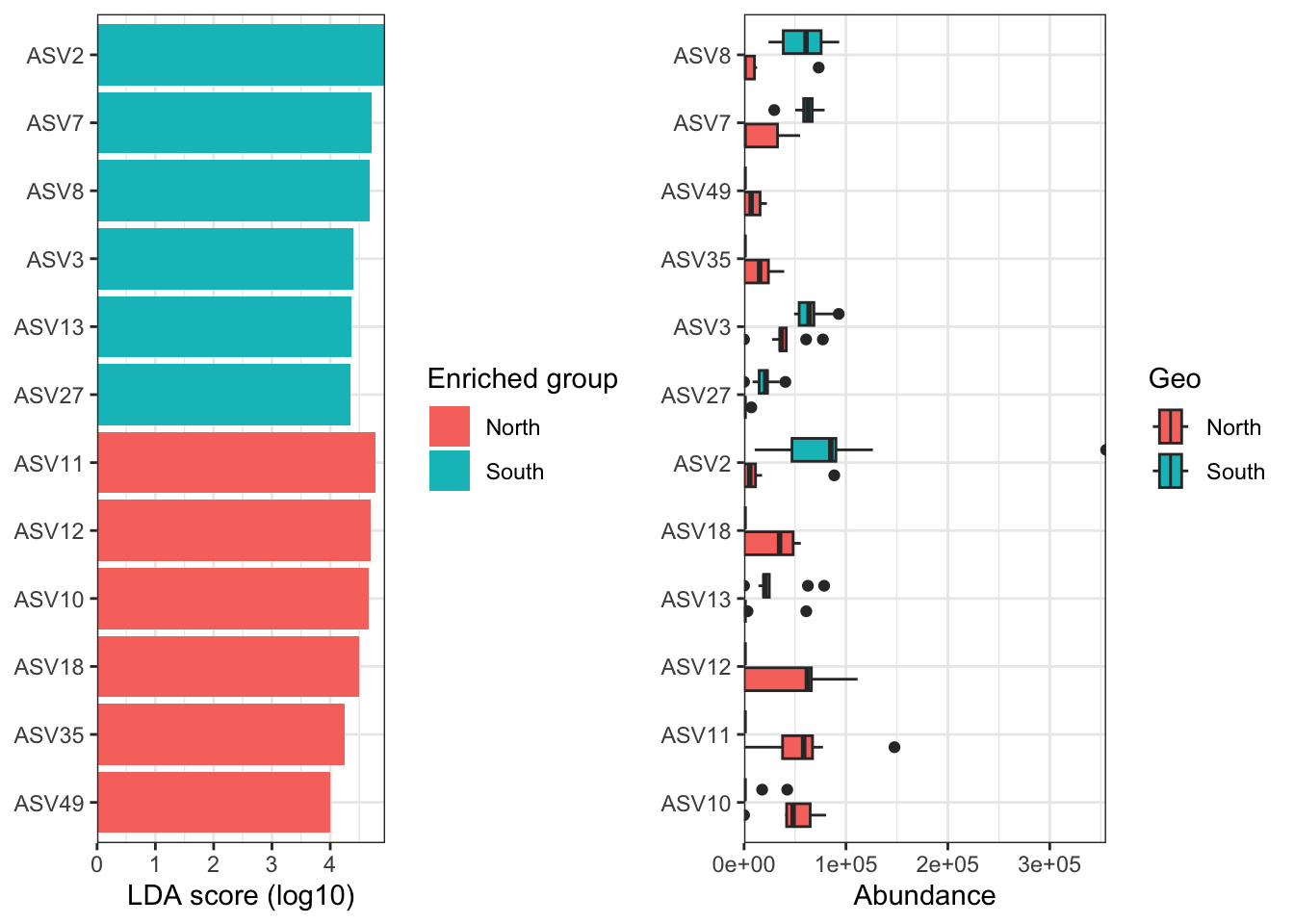
LEFse identifies 12 biomarkers and among them ASV 7, 11 and 12 that we already identifies ealier with other methods.
The ANCOM-BC methodology assumes that the observed sample is an unknown fraction of a unit volume of the ecosystem, and the sampling fraction varies from sample to sample. ANCOM-BC accounts for sampling fraction by introducing a sample-specific offset term in a linear regression framework, that is estimated from the observed data. The offset term serves as the bias correction, and the linear regression framework in log scale is analogous to log-ratio transformation to deal with the compositionality of microbiome data. Furthermore, this method provides p-values and confidence intervals for each taxon. It also controls the FDR and it is computationally simple to implement.
#ancomBC be careful you have to use the RAW data (physeq)!!!!!
mm_ancombc <- run_ancombc_patched(physeq, group = "Geo",
                                            taxa_rank = "none",
                                            pvalue_cutoff = 0.001,
                                            p_adjust = "fdr")

mm_ancombc_table <- data.frame(mm_ancombc@marker_table)
mm_ancombc_table
feature enrich_group ef_W pvalue padj
marker1 ASV2 South 3.980197 6.885820e-05 7.230111e-04
marker2 ASV7 South 4.341347 1.416118e-05 1.652137e-04
marker3 ASV8 South 4.532481 5.829496e-06 1.020162e-04
marker4 ASV10 North -4.775089 1.796277e-06 6.286968e-05
marker5 ASV11 North -5.811580 6.188594e-09 3.249012e-07
marker6 ASV12 North -4.466839 7.938375e-06 1.041912e-04
marker7 ASV18 North -4.561024 5.090471e-06 1.020162e-04
marker8 ASV27 South 5.874154 4.250091e-09 3.249012e-07
marker9 ASV35 North -4.483869 7.330158e-06 1.041912e-04
marker10 ASV49 North -4.680720 2.858686e-06 7.504051e-05an_ef <- microbiomeMarker::plot_ef_bar(mm_ancombc)
an_abd <- microbiomeMarker::plot_abundance(mm_ancombc, group = "Geo")
gridExtra::grid.arrange(an_ef, an_abd, nrow = 1)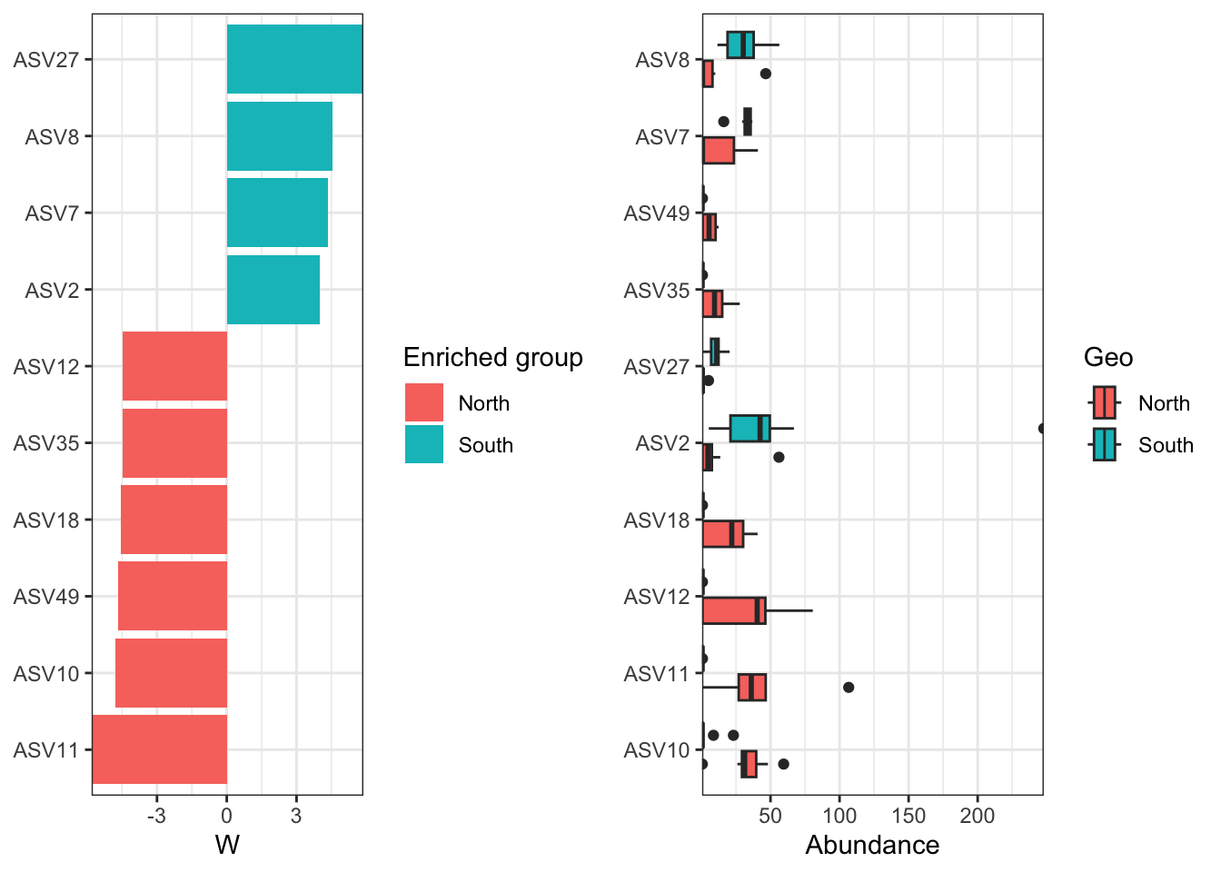
ANCOM-BC identifies 10 biomarkers and all in common with the results of the LEFse analysis.